Table of Contents
- Preface
- I. Introduction
- II. Vectors
- III. Tensors of Rank > 1
- IV. Covariant Derivative
Preface
These are my notes on tensors. Like many pages on my site, they are not meant to be an exhaustive treatise, but instead, emphasize topics – including proofs – that I would like to remember or that are needed for other pages on the site.
This page draws from a number of resources. Here are the main three:
- eigenchris. Tensors For Beginners . YouTube, 10 Dec. 2017, https://www.youtube.com/watch?v=8ptMTLzV4-I&list=PLJHszsWbB6hrkmmq57lX8BV-o-YIOFsiG&index=1. : This is an free 18 part video series that goes into considerable detail regarding the tensor theory. However, the explanations are excellent, moving methodically through topics step-by-step. It does, however, assume basic familiarity with linear algebra.
- Collier, Peter. A Most Incomprehensible Thing. Incomprehensible Books, 2017. : Directed toward the interested amateur. Step-by-step derivations. Bargain price – Amazon Kindle version for $3.99.
- Fleisch, Daniel A. A Student’s Guide to Vectors and Tensors. Cambridge University Press, 2011. : Great Book geared toward undergraduate math and science students. This article is based most on this reference. Amazon Kindle version for $23.99. Well worth the money.
To navigate this page, click on a link in the table of contents and it will bring you to the specified section. Clicking on the title of a section will bring you back to the table of contents.
Regarding explanatory information, clicking on the button (often labeled “here”) for the explanatory note will unhide it. To re-hide the information, click again on the button that opened it.
I. Introduction
Tensors are mathematical objects that are widely used largely because they do not change under coordinate changes. This is important in a number of disciplines but is particularly critical in physics. Why? Because the laws of physics are thought to be invariant irrespective of the coordinate system being employed. This is particularly crucial in special and general relativity. They are helpful in understanding complex (nonEuclidean) geometry as well.
So what are tensors? There are several definitions.
- A multidimensional array (or grid) of numbers: Practical but misses out on geometric meaning of tensors.
- A mathematical object that is invariant under coordinate changes and which transform under coordinate changes in specific, predicable ways
- A collection of vectors and covectors combined together under the tensor product
Hopefully, the meaning of these definitions will become clear as we go along.
From our first definition, we can come up with a classification of tensors. Tensors can be classified by the number of indices contained by each entry in the grid that makes up the tensor. That number of indices is referred to as the tensor’s rank. Each index can specify an unlimited number of dimensions. Up to rank 3, we can think of the number of indices as the number of directions the grid extends into.
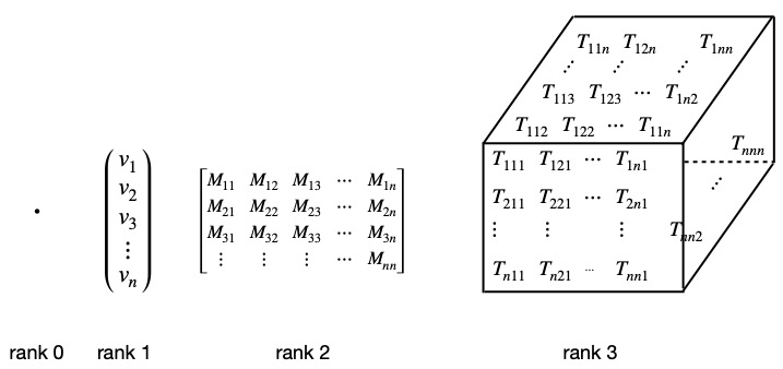
Figure I.1 shows some examples of tensors that provides some intuition regarding how they are categorized.
A rank 0 tensor is just a number, also called a scalar. It doesn’t extend in any direction; it just sits at a single point on a graph.
Rank 1 tensors are vectors. They consist of just 1 column or 1 row of numbers extending out in one direction. The number of entries in that column or row specifies the number of dimensions of the vector.
Rank 2 tensors are analogous to matrices, arrays (or grids) of numbers that extend in two directions – along rows and columns. Note, however, that matrices are just collections of numbers. To specify a rank 2 tensor, we also need to specify the basis vectors we are using.
Rank 3 tensors would extend in three directions, like a Rubik’s Cube. Each block in the Rubik’s Cube can be thought of as containing a number.
Tensors of higher rank are harder to visualize (because we live in a 3-dimensional world) but you can imagine that we could put more numbers into more directions. For example, the Riemann curvature tensor used in general relativity has 4 indices and each index species 4 spacetime dimensions (1 dimension of time and 3 different dimensions of space). Thus, this mathematical object contains 256 pieces of information, or components –  – (although only 20 of those components are independent).
II. Vectors
Vectors – rank 1 tensors – are a good starting point to examine the properties of tensors.
I introduced vectors in my page on linear algebra; I won’t rehash that here. Instead, in this article, I’ll expand on what I’ve discussed previously. I talked about the dot product of vectors in the vector section of my linear algebra page. We’ll start here by discuss some other important operations that can be performed vectors. The first is the curl.
II.A Curl
In my page on linear algebra, I discussed one method of multiplying vectors, the dot product, which, when applied, yields a scalar. A second method of multiplying vectors, the curl, by contrast, yields another vector. The curl of two vectors  and
and  , is defined as follows:

where
î, ĵ and k̂ are unit vectors in the x, y and z directions of a classic Euclidean coordinate system.
The curl can also be written as a determinant:
![\[\vec{A} \times \vec{B} = \begin{vmatrix}\hat{i} & \hat{j} & \hat{k}\\ A_x & A_y & A_z\\ B_x & B_y & B_z\end{vmatrix}\quad \text{eq (2)}\]](https://www.samartigliere.com/wp-content/ql-cache/quicklatex.com-cbe23d6c586fe200876e3d4c1253c723_l3.png "Rendered by QuickLaTeX.com")
To obtain the same expression as eq (1) using the determinant, we employed the cofactor formula. You can find more information on determinants in general, and the cofactor formula specifically, on my linear algebra page.
We said that the product of the curl is a vector. Therefore, it must have a direction. That direction is perpendicular to the plane of the vectors whose product is being taken. Of course, there are two possible directions that can be perpendicular to a plane. Which one is the correct direction? The correct direction is give by what’s called the right hand rule. The right hand rule has several forms. The one I like best is the one I consider the simplest and is depicted in figure II.A.1:
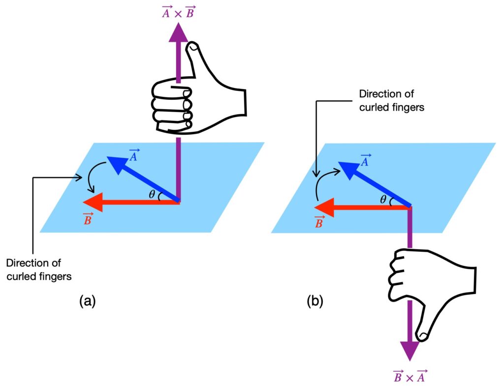
To determine the direction of product of the curl, we curl our fingers from the first vector toward in the curl expression toward the second. For example, if our curl is  , as in figure II.A.1a, we place the pinky-side of part of our right hand on and curl the tips of our fingers toward . Our thumb points upward; that’s the direction of the curl’s resultant vector. In figure 1b, we place the index finger-side of our hand on the first vector in our curl expression, , and curl our finger tips toward . When we do this, we get our resultant vector direction: in this case, downward.
The magnitude of the curl is also given by:
![\[ \lvert \lvert \vec{A} \times \vec{B} \rvert \rvert= \lvert \lvert \vec{A}\rvert \rvert\,\lvert \lvert \vec{B}\rvert \rvert \sin\theta \quad \text{eq (3)}\]](https://www.samartigliere.com/wp-content/ql-cache/quicklatex.com-b34173cfd39928d7054d835d5d66acf1_l3.png "Rendered by QuickLaTeX.com")
A proof of this, taken from Khan Academy, can be seen by clicking .
 and
and 


![\[\begin{matrix}a_1^2(b_1^2+b_2^2+b_3^2)\\ +a_2^2(b_1^2+b_2^2+b_3^2)\\+a_3^2(b_1^2+b_2^2+b_3^2) \end{matrix}=\underbrace{(b_1^2+b_2^2+b_3^2)}_{\lvert\lvert \vec{B}\rvert\rvert^2}\underbrace{(a_1^2+a_2^2+a_3^2)}_{\lvert\lvert \vec{A}\rvert\rvert^2}\]](https://www.samartigliere.com/wp-content/ql-cache/quicklatex.com-718b85da6300db6ec9c0d58300e7de56_l3.png "Rendered by QuickLaTeX.com")
![\[\lvert\lvert\vec{A}\times\vec{B}\rvert \rvert^2+\lvert\lvert\vec{A}\rvert\rvert^2\,\lvert\lvert\vec{A}\rvert\rvert^2 \cos^2\theta&=\lvert\lvert \vec{A}\rvert\rvert^2\,\lvert\lvert \vec{B}\rvert\rvert^2\]](https://www.samartigliere.com/wp-content/ql-cache/quicklatex.com-fa37e5060092c53069f8f8d25437a3f0_l3.png "Rendered by QuickLaTeX.com")

![\[ \sin^2\theta + \cos^2\theta = 1 \quad \Rightarrow \quad \sin^2\theta = 1-\cos^2\theta\]](https://www.samartigliere.com/wp-content/ql-cache/quicklatex.com-8c72f780a9f23125501c850911588df7_l3.png "Rendered by QuickLaTeX.com")
![\[ \lvert\lvert\vec{A}\times\vec{B}\rvert \rvert^2&=\lvert\lvert \vec{A}\rvert\rvert^2\,\lvert\lvert \vec{B}\rvert\rvert^2\sin^2\theta \]](https://www.samartigliere.com/wp-content/ql-cache/quicklatex.com-8b002fdba5347a11ed4b5f3860c5b20e_l3.png "Rendered by QuickLaTeX.com")
![\[ \lvert\lvert\vec{A}\times\vec{B}\rvert \rvert&=\lvert\lvert \vec{A}\rvert\rvert\,\lvert\lvert \vec{B}\rvert\rvert\sin\theta \]](https://www.samartigliere.com/wp-content/ql-cache/quicklatex.com-18289a19fff37d5b9a0a519163a8c5b9_l3.png "Rendered by QuickLaTeX.com")
Another interesting fact related to the curl is that the magnitude of the curl equals the area formed from a parallelogram made from the two vectors that contribute to the curl. Figure 2 helps us see why.
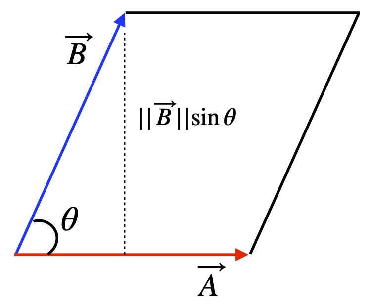
In figure II.A.2, we have two vectors, and at angle  to each other. We can extent line segments outward from the tips of both vectors to form a parallelogram. We then drop a perpendicular from the tip of to . This perpendicular segment represents the height of the parallelogram we made. We know that the area of a parallelogram is base times height which, in this case is
  . But we saw above that is just
  .
.
II.B Triple Scalar Product
The triple scalar product, for three vectors , and  , is defined as
![\[\vec{A}\cdot(\vec{B}\times\vec{C})\]](https://www.samartigliere.com/wp-content/ql-cache/quicklatex.com-42f06a3bc69d84ab40d209272eb69b6d_l3.png "Rendered by QuickLaTeX.com")
Since the curl produces a vector, then we’re taking the dot product of that resultant vector with another vector (in this case, ), the result is a scalar.
One way to express the triple scalar product is:

Another handy way to write the triple scalar product is:
![\[ \vec{A} \cdot (\vec{B} \times \vec{C}) = \begin{vmatrix} A_x & A_y & A_z\\ B_x & B_y & B_z\\ C_x & C_y & C_z\\ \end{vmatrix}\quad \text{eq (5)}\]](https://www.samartigliere.com/wp-content/ql-cache/quicklatex.com-df9c588fcd4e6321cdde169f21220e66_l3.png "Rendered by QuickLaTeX.com")
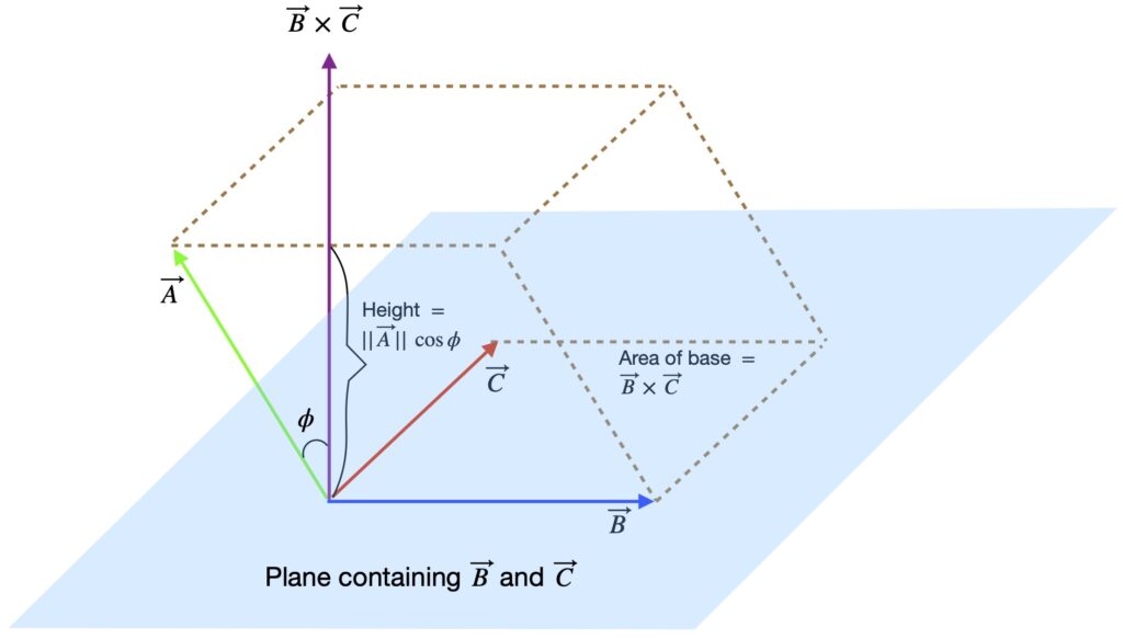
Note, also, that the volume of the parallelepiped formed by the three vectors that make up the triple scalar product is given by the triple scalar product (figure II.B.1).
II.C Triple vector product
To be added.
II.D Gradient
![\[ \nabla \phi = \frac{\partial \phi}{\partial x}\hat{e}_x + \frac{\partial \phi}{\partial y}\hat{e}_y + \frac{\partial \phi}{\partial z}\hat{e}_z \]](https://www.samartigliere.com/wp-content/ql-cache/quicklatex.com-cc5f45dfd8f0638ff2aabde0680372ca_l3.png "Rendered by QuickLaTeX.com")
where
 is the symbol for the gradient
 is a scalar field
 is a unit vector in the ith direction
The result of the gradient is a vector field.
II.E Divergence
For a vector field
![\[ \vec{V}=V^x\hat{e}_x + V^y\hat{e}_y + V^z\hat{e}_z + \]](https://www.samartigliere.com/wp-content/ql-cache/quicklatex.com-fccf0ed7bcf214633b5ad82501143dc2_l3.png "Rendered by QuickLaTeX.com")
The divergence is:
![\[ \nabla \cdot \vec{V} = \frac{\partial V^x}{\partial x} + \frac{\partial V^y}{\partial y} + \frac{\partial V^z}{\partial z} \]](https://www.samartigliere.com/wp-content/ql-cache/quicklatex.com-4256e91bc1e4a5c6888c9471768b39bb_l3.png "Rendered by QuickLaTeX.com")
The result of the divergence is a scalar.
II.F Laplacian
If  is the gradient of a scalar field, , then the Laplacian is:
![\[ \nabla \cdot \vec{V} = \nabla \cdot \nabla \phi = \nabla^2 \phi = \frac{\partial^2 \phi}{\partial x^2} + \frac{\partial^2 \phi}{\partial y^2} + \frac{\partial^2 \phi}{\partial z^2} \]](https://www.samartigliere.com/wp-content/ql-cache/quicklatex.com-00b67e4fb94288144f688de7c42f1f15_l3.png "Rendered by QuickLaTeX.com")
The result of the Laplacian is a scalar.
II.G Vector Identities
II.G.1 CAB-BAC Identity
This identity states that the curl of the curl equals the gradient of the divergence minus the Laplacian. The formula is:
![\[ \nabla \times (\nabla \times \vec{V}) = \nabla(\nabla \cdot \vec{V}) - \nabla^2\vec{V} \]](https://www.samartigliere.com/wp-content/ql-cache/quicklatex.com-f8b387a53d1f711db992033cb6ace489_l3.png "Rendered by QuickLaTeX.com")
Divergence of the Curl is Zero


 . Thus, we’re left with:

 ,
,  and
and  “disappear” when the divergence is taken. This is because we’re taking the dot product of 2 vectors – the partial derivative operator and the unit vector – and the dot product of 2 vectors is a scalar. Specifically, in this case, the unit vector is in “the same direction” as the partial derivative. Therefore, the value of the partial derivative dotted with the unit vector is 1 (e.g.
  ).
).Curl of the Divergence is Zero
 be a scalar field. Then:


II.H Contravariant vs Covariant
The vectors discussed on my linear algebra page and the vectors we’ve discussed so far here are the classic vectors you may have learned about in high school – arrows that have a magnitude and direction in Euclidean space – a space where coordinate axes are at right angles and where spacing between units on these axes is the same everywhere. We can describe such vectors with components, numbers that tell us how many units we have to travel in each direction to get from the beginning of the vector to its end, as shown in figure II.H.1.
Furthermore, we can write these vectors as follows :
![\[ \vec{A} = \vec{A^x} + \vec{A^y} = A^x\vec{e_x} + A^y\vec{e_y}\quad \text{eq (6)}\]](https://www.samartigliere.com/wp-content/ql-cache/quicklatex.com-3fa834b8d5ccbda4fa4b9ab9136cc33d_l3.png "Rendered by QuickLaTeX.com")
 and
and  are component vectors of which, when added tip to tail, yield
  and are basis vectors, 1 unit in length, pointing in the x and y directions, respectively
 and
and  are the magnitudes of the component vectors and ; we simply call them the components of
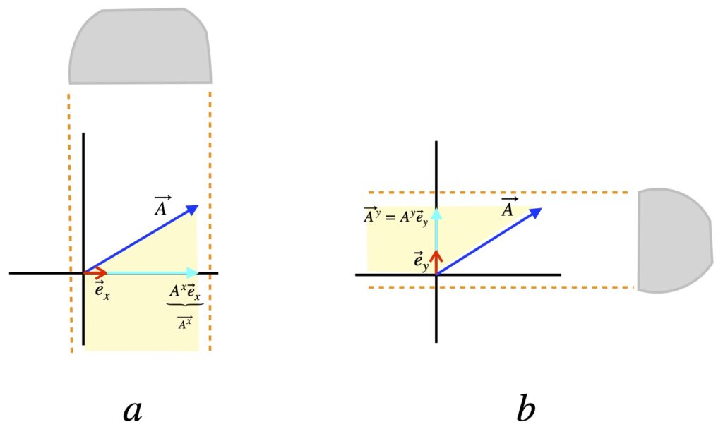
Figure II.H.1, patterned after a diagram in Dan Fleisch’s text, shows how we can find the coordinates of a vector in Euclidean space. To find , we imagine shining a light perpendicular to the x-axis, or equivalently, parallel to the y-axis. The shadow it makes on the x-axis is  . And since is the magnitude of , is the length of .
Likewise, to find , we imagine shining a light perpendicular to the y-axis, or equivalently, parallel to the x-axis. The shadow it makes on the y-axis is  . And since is the magnitude of , is the length of .
Notice that the components and component vectors contain superscripts and basis vectors have a subscripts. We’ll come back to this.
For now, let’s see how the components of transform under coordinate transformations. Let’s look specifically at the case of coordinate system rotation and its effect on components and basis vectors.
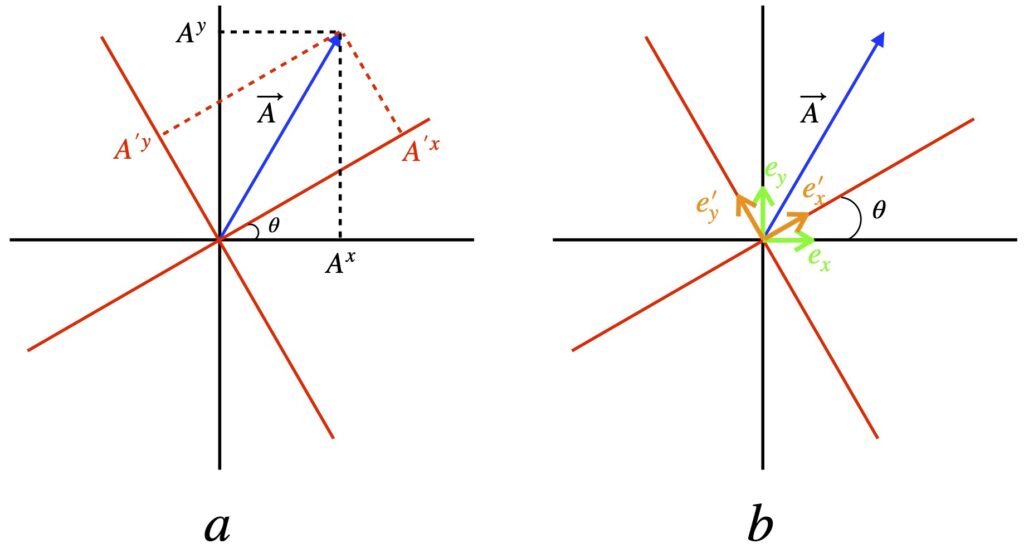
In figure II.H.2, the black axes are the coordinates before transformation and the red axes are the coordinate system after a 30° counterclockwise rotation. Figure II.H.2a shows the effect of coordinate rotation on vector components while figure II.H.2b shows the effect on basis vectors. Two things are evident.
- The vector does not change with coordinate rotation
- The components of do change with coordinate rotation
It turns out that vector components transform by what Dan Fleisch calls the indirect matrix and what the eigenchris website calls the backward transformation matrix:

One can find additional information elsewhere on this website regarding the effect of coordinate rotation on vector components and matrix multiplication.1
Of course, we know that vectors aren’t made of just components; they’re a combination of components and basis vectors. Therefore, when a vector is transformed from one coordinate system to another, one must transform not only the components, but also the basis vectors. In contrast to the way new vector components transform, basis vectors are transformed by multiplication by the inverse of the matrix used for the indirect or backward transformation. We’ll call this matrix the direct (per Fleisch) or forward (per eigenchris) transformation matrix. In the case of coordinate axis rotation, as we might expect, this matrix is the same as the matrix that finds new coordinates for a vector that’s rotated while keeping the coordinates still.

And this makes sense because that’s exactly what we’re doing: rotating the basis vectors. More details about this can be found in the section entitled Basis vector rotation in Cartesian coordinates on my page on coordinate transformations.
I mentioned above that the direct/forward transformation matrix is the inverse of the indirect/backward matrix:


Why is this important? Because when we transform both the components and the basis vectors of a vector using these matrices, we get the same vector from which we started:


In short, this means that while vector components and basis vectors are modified by a coordinate transformation, the vector, itself, remains unchanged – just as figure II.H.2 suggests.
Notice that we’ve been using superscripts for vector components and subscripts for basis vectors. To see why, consider situations where the axes of the coordinate system being used are not parallel to each other or the length of units on these axes are not uniform from place to place. Let’s look at the first situation (figure II.H.3).
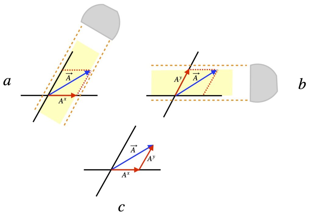
Unlike the so-called orthonormal basis we’ve been working with so far, when axes are not orthogonal, there are two ways one can determine vector components. The first is shown in figure II.H.3. As described in Dan Fleisch’s book, in what we’ll call the parallel method, the x-component is represented by the shadow made when one shines a light parallel to the y-axis (figure II.H.3a). And the y-component of a vector is represented by the shadow formed when one shines a light parallel to the x-axis (figure II.H.3b). Figure II.H.3c shows that the components formed in this manner add together to form in the same way that vector components added to make a vector when we used an orthonormal basis. If we were to change coordinate systems, the components would transform using the backward transformation matrix and the basis vectors would change using the forward matrix. The ensuing proof of this is patterned after the eignenchris tensor video series, especially https://www.youtube.com/watch?v=bpuE_XmWQ8Y.
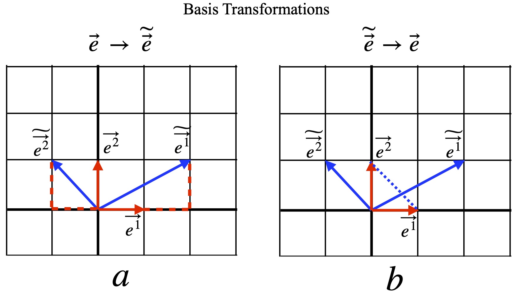
We consider two vector bases, as depicted in figure II.H.4. We start with the basis  and
and  , shown in red. We want to describe the basis
  and
and  (displayed in blue) in terms of
  and
and  . We can see from figure II.H.4a that:


We can write this in matrix form:

We’ll call  the forward transformation matrix.
We can generalize the transformation equation for the basis vectors. For the 2-dimensional case:


where 
For the n-dimensional case:


where 
We can write this in more compact form using summation notation:

Next, we want to get the  components in terms of the
  components. From figure II.H.4b, we can see that:


We can put this in matrix form as well:

We’ll refer to  as the backward transformation matrix. We can generalize the
  transformation by using the same process as we used above and write it utilizing summation notation, as follows:

If we multiply the forward and backward matrices together, the result is the identity matrix:


That means that the forward and backward matrices are inverses of each other.
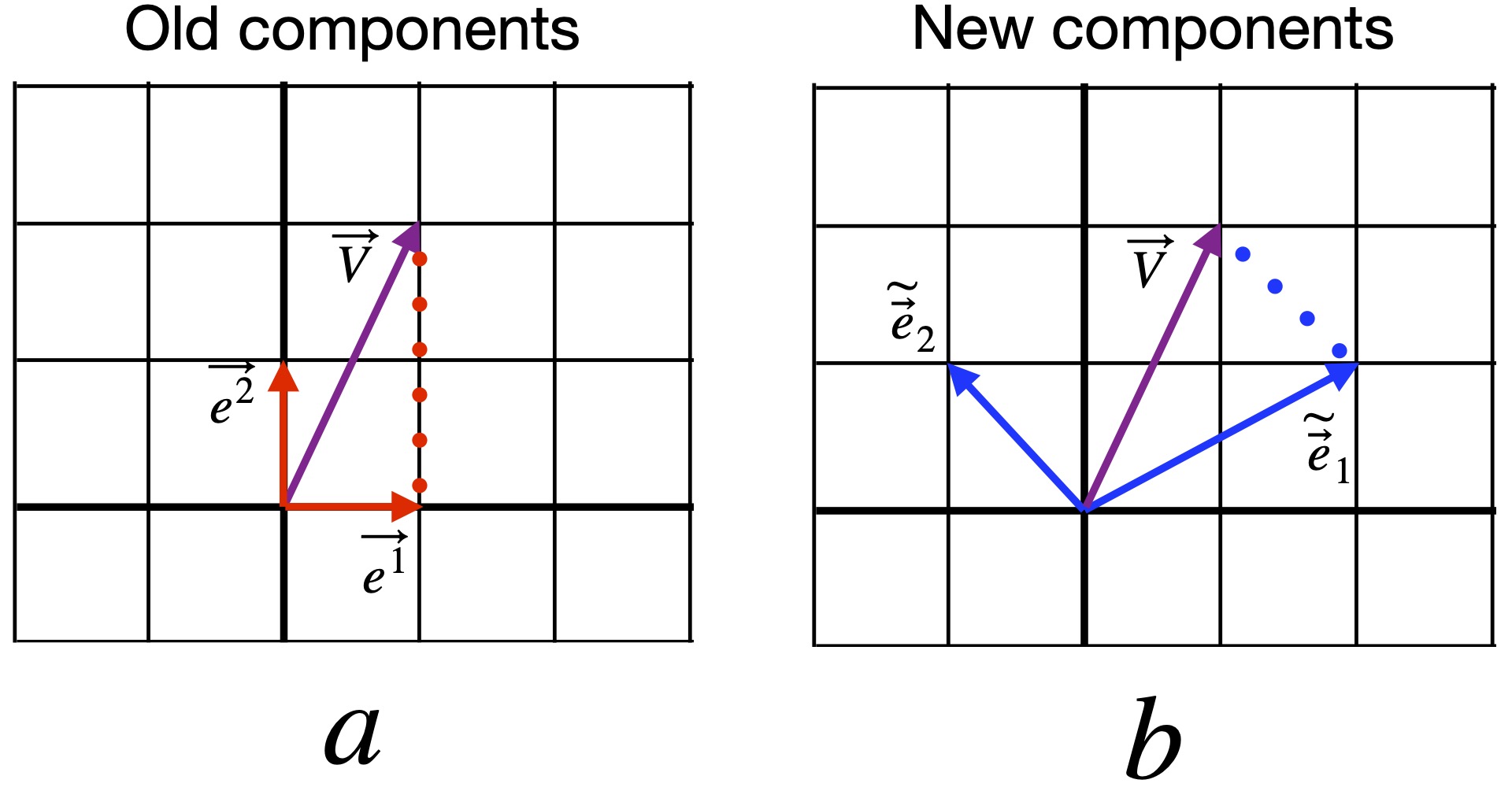
Our next tasks are 1) to find the components of vector in the basis (we’ll call them the old componenents) and the basis (we’ll call them the new componenents) and 2) to see how the two sets of components relate to each other
From figure II.H.5a, we see that the components of vector in the basis are  .
.
From figure II.H.5b, we see that the components of vector in the  basis are
  .
.
So how are the two sets of components related? Well, to make things work out, if we start with components in the basis, and want to know the components in the basis, we have:


![=\left[V^1(\frac13) + V^2(\frac13)\right]\widetilde{\vec{e}}_{\,1} + \left[V^1(-\frac13) + V^2(\frac23)\right]\widetilde{\vec{e}}_{\,2}](https://www.samartigliere.com/wp-content/ql-cache/quicklatex.com-6c1f3ced399976986ae08462a25053fc_l3.png "Rendered by QuickLaTeX.com")
We can break this down into two equations. First:
![\widetilde{V}^1\widetilde{\vec{e}}_{\,1}= \left[V^1(\frac13) + V^2(\frac13)\right]\widetilde{\vec{e}}_{\,1}\,\,\Rightarrow\,\,\widetilde{V}^1=V^1(\frac13) + V^2(\frac13)](https://www.samartigliere.com/wp-content/ql-cache/quicklatex.com-c062b200473adce5936e69c3f66606e9_l3.png "Rendered by QuickLaTeX.com")
and
![\widetilde{V}^2\widetilde{\vec{e}}_2=\left[V^1(-\frac13) + V^2(\frac23)\right]\widetilde{\vec{e}}_{\,2}\,\,\Rightarrow\,\,\widetilde{V}^2=V^1(-\frac13) + V^2(\frac23)](https://www.samartigliere.com/wp-content/ql-cache/quicklatex.com-ea69f0b33bef3acea60ac61ce4b3d1b0_l3.png "Rendered by QuickLaTeX.com")
We can recombine these equations into matrix form:

We can check to see if this agrees with the values for  ,
,  ,
,  and
and  we got from figure 6.2:

Indeed they do.
We can generalize the above transformation equation in a manner similar to what we’ve done before and express it with summation notation like so:

Transformation of the new components into the old ones follows an analogous process. The steps are:
Write as a linear combination of the and bases, then make the appropriate substitutions:


![=\left[\widetilde{V}^1 (2) + \widetilde{V}^2(-1)\right]\vec{e}_1 + \left[\widetilde{V}^1 (1) + \widetilde{V}^2 (1)\right]\vec{e}_2](https://www.samartigliere.com/wp-content/ql-cache/quicklatex.com-692b46e42836d0b1c151b40cb259b876_l3.png "Rendered by QuickLaTeX.com")
Break this equation down into two equations:
![V^1\vec{e}_1=\left[\widetilde{V}^1 (2) + \widetilde{V}^2(-1)\right]\vec{e}_1\,\,\Rightarrow\,\,V^1=\widetilde{V}^1 (2) + \widetilde{V}^2(-1)](https://www.samartigliere.com/wp-content/ql-cache/quicklatex.com-0876eb2acfb301f0432f839372ec294b_l3.png "Rendered by QuickLaTeX.com")
and
![V^2\vec{e}_2=\left[\widetilde{V}^1 (1) + \widetilde{V}^2 (1)\right]\vec{e}_2\,\,\Rightarrow\,\,V^2=\widetilde{V}^1 (1) + \widetilde{V}^2 (1)](https://www.samartigliere.com/wp-content/ql-cache/quicklatex.com-4fc29906646db85d49e18de80056d88f_l3.png "Rendered by QuickLaTeX.com")
Recombine these two equations into matrix form:

Confirm that this agrees with the values for the components we got from figure II.H.5:

The summation equation for the  transformation is:

I think it’s instructive to look at the long versions of the proofs about how basis vectors and components transform. However, there’s a much easier way to derive these transformations using linear algebra. If we start with the vector, , we know that to obtain  we apply the backward transformation matrix,
  :
:

Applying the inverse of to both sides of this equation, we obtain:

But we know that  and
and  is the forward matrix,
  . So
. So

Notice that the transformation matrices used to relate old and new components are opposite to the transformation matrices used to transform their corresponding basis vectors:
Old basis vectors  New basis vectors
Old components  New components
New basis vectors Old basis vectors
New components Old components
That’s why they’re called contravariant components.
Note, also, that we use a row vector and subscripts when manipulating the basis vectors as opposed to column vectors and superscripts when dealing with components, suggesting the two are intrinsically different entities.
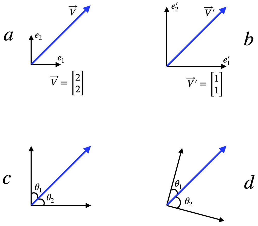
As a consequence of components and basis vectors transforming in opposite ways, the length of components decrease as basis vector component length increases, and vice versa. This is depicted in figure II.H.6a and II.H.6b. Figure II.H.6c and II.H.6d provide further intuition regarding the origin of the name “contravariant.” In figure II.H.6c, we can see that angles  and
and  are equal. If the coordinate system is rotated clockwise (figure II.H.6d), then, relative to the new coordinate axes, appears to rotate counterclockwise i.e., contrary to the basis vector rotation.
By convention, superscripts are used to designate contravariant components and subscripts are used for the basis vectors by which they are multiplied.
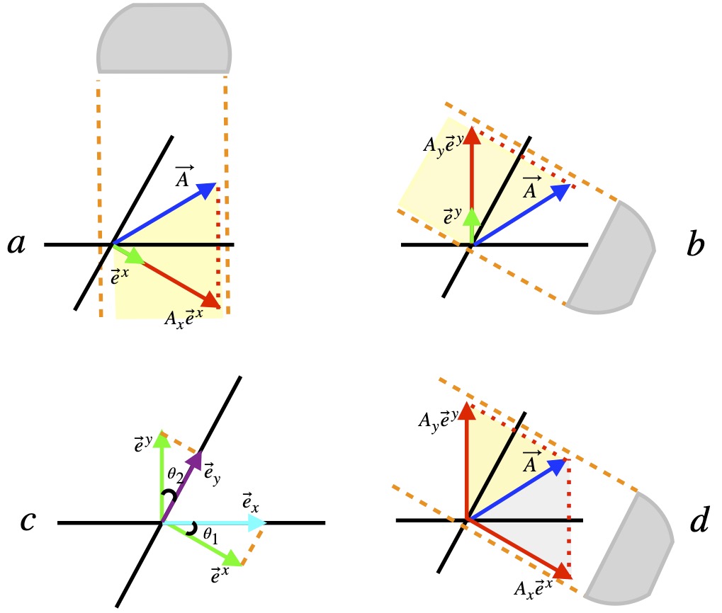
All of the component transformations we’ve talked about so far apply when the parallel method of evaluating vector components is employed. But the parallel method isn’t the only method available. As shown in figure II.H.7, we can also obtain x-components by shining a light perpendicular to the x-axis. Likewise, to find the y-components, we shine our light perpendicular to the y-axis.
We can see that components created in this way are different than those created by the parallel method. In addition, figure II.H.7 shows us that if we try to add vector components – made by the perpendicular method – by applying the technique that we used for vectors in Cartesian coordinates or those derived from the parallel projection method, it doesn’t work. Still, we can’t help but believe that there has to be some way to make “components” from the perpendicular method. After all, from what vantage point we look at the axes shouldn’t matter. In fact, there is.
What we need to do is to use different basis vectors. This is shown in figure II.H.8.
There are 2 defining characteristics of these new basis vectors which are called dual basis vectors:
- Each dual basis vector must be be perpendicular to all original basis vectors with different indices. This is evident in figure II.H.8c (i.e.,
 is perpendicular to
  and
and  is perpendicular to
  ). Another way to say this is
  and
and  .
. - The dot product of a dual basis vector with a original basis vector with the same index equals 1. Thus, in the figure II.H.8c
 and
and  .
. - More generally, we can write this as
 where
where 
From figure II.H.8c, it’s harder to see, at least for me, why this second definition is true. We can see that and are separated by an angle and can be thought of as sides of a right triangle. From this, we know that:

From the second definition above, we have:

These two equations are difficult to reconcile except when  . If anyone can better explain the connection between the second definition for dual basis vectors and the perpendicular method for obtaining these vectors, please leave a comment.
Evident from figure II.H.8d, though, is that if we make our perpendicular projections onto the direction defined by the dual basis vectors, the resulting vectors add up to make . That is, they add as components. To see an example with calculations, click .
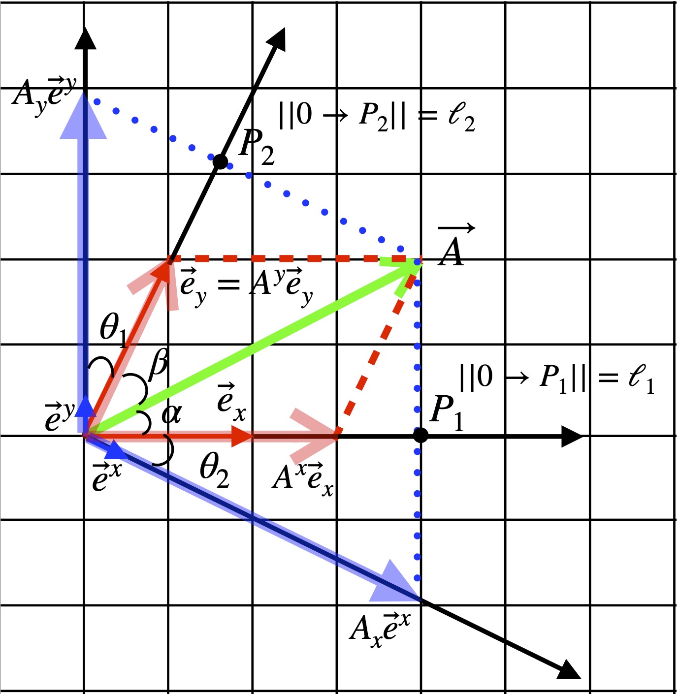


 , we have to find
  . To do this, we need to recognize that 1) the line segment between the origin and point
  2) the line segment between
  and the tip of
  and 3) the vector
  as
as  . We know that
  and
and  Then:
Then:

 , we have to find
  . To do this, we need to recognize that 1) the line segment between the origin and the and point
  2) the line segment between
  and the tip of
  and 3) the vector
  as
as  . We can calculate
  by recognizing that 1) the line segment
  ) is given by
  Then:
Then:


The components combined with dual basis vectors to create vector components are called covariant components, and to distinguish them from contravariant components, subscripts are used to designate them. Similarly, to distinguish dual basis vectors from the basis vectors that multiply contravariant components, superscripts are used.
To understand why covariant components get their name, we need to see how covector components and the basis vectors they’re multiplied by to obtain a covector actually transform. Here’s a summary:


where
 and
and  are the covector components
 and
and  are the basis vectors for the dual vector space
 are the components of the forward transformation matrix
 are the components of the forward transformation matrix
[For a proof of these expressions, patterned after the eigenchris videos (especially https://www.youtube.com/watch?v=d5da-mcVJ20), click .]
 for the dual vector space,
  from the old basis vectors,
  , for that space,
 :
:
 . In addition, we’ve previously shown that
  . We can refer to indices by whatever letters we want so
  Substituting, we get:<\p>


 . Thus:
 except when
  so the only time the expression
  is when
  . Taking this into account, we have:
 . That means that Q_{ij} = B_{ij}. When we substitute this into the equation we started out with,
  . We end up with:


 is the identity matrix so
 . Therefore:

 :
:


 in the equation from which we started gives us:
 but our linear algebra proof is quicker:


 transforms via the backward transformation matrix.
Components of covectors are called covariant because their manner of transformation from old to new components “coincides” with (transforms in the same way as) that of basis vectors; they both use the forward transformation:
 and
and 
And in contrast to contravariant components, if dual basis vector length is increased, then the length of its associated covariant component is also increased. Likewise, when dual basis vectors are rotated in a given direction, the vector appears to rotate in the same direction (versus what’s shown in figure II.H.6c and II.H.6d).
Note that many authors refer to vectors as being contravariant or covariant, but strictly speaking, the vector itself (being a tensor) is an invariant object which can be described using either contravariant or covariant components.
Many matheticians now consider the terms contravariant and covariant to be outdated. More modern terminologies include calling vectors with contravariant components vectors and vectors with covariant components covectors, linear functionals or one-forms. The reason for this, they say, is that the mathematical objects they are calling covectors or one-forms are fundamentally different from vectors. They see them as operators that take in a vector as an argument and spit out a scalar:
 where
where  is the covector/one-form, acting as an operator, and
  is a scalar (i.e. a number).
They also follow linearity:


where
 is a covector
 and
and  are vectors on which the covector operates
 is a scalar
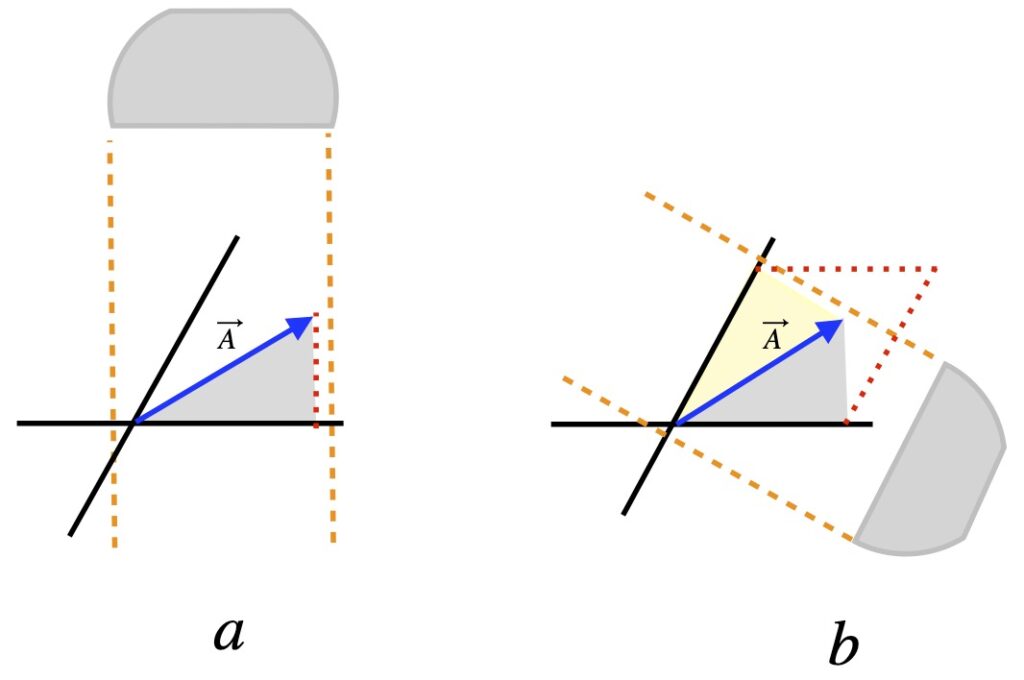
In this scheme, these operators (or covectors or one-forms or whatever you want to call them) form a separate a separate vector space that’s referred to as a dual space. Furthermore, they visualize these covectors as a series of hyperplanes – or simple 2-dimensional planes if we’re dealing with just 2 dimensions, like we’ve been dealing with in the examples I’ve given – perpendicular to the direction of the dual basis vectors. The components of the covector, then, are given by the number of hyperplanes that are “pierced” in moving in the direction of the dual basis vector to the point where the perpendicular projection of the vector intersects the axes formed by the dual basis vector. Now, that’s a mouthful. Hopefully, figure II.H.9, which applies this alternate viewpoint to the example given in figure II.H.8, will clarify things.
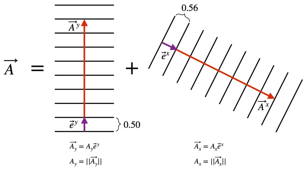
In figure II.H.9, we see noted in figure II.H.8 expressed with covariant components and dual basis vectors. The parallel black lines represent hyperplanes running in and out of the plane of the screen. The number of hyperplanes traversed by the component vectors represent the component vector magnitudes.
There are definitely situations where this hyperplane picture is helpful such as application of Stokes theorem. However, for me at least, seeing the hyperplanes as tick marks on an axis works fairly well.
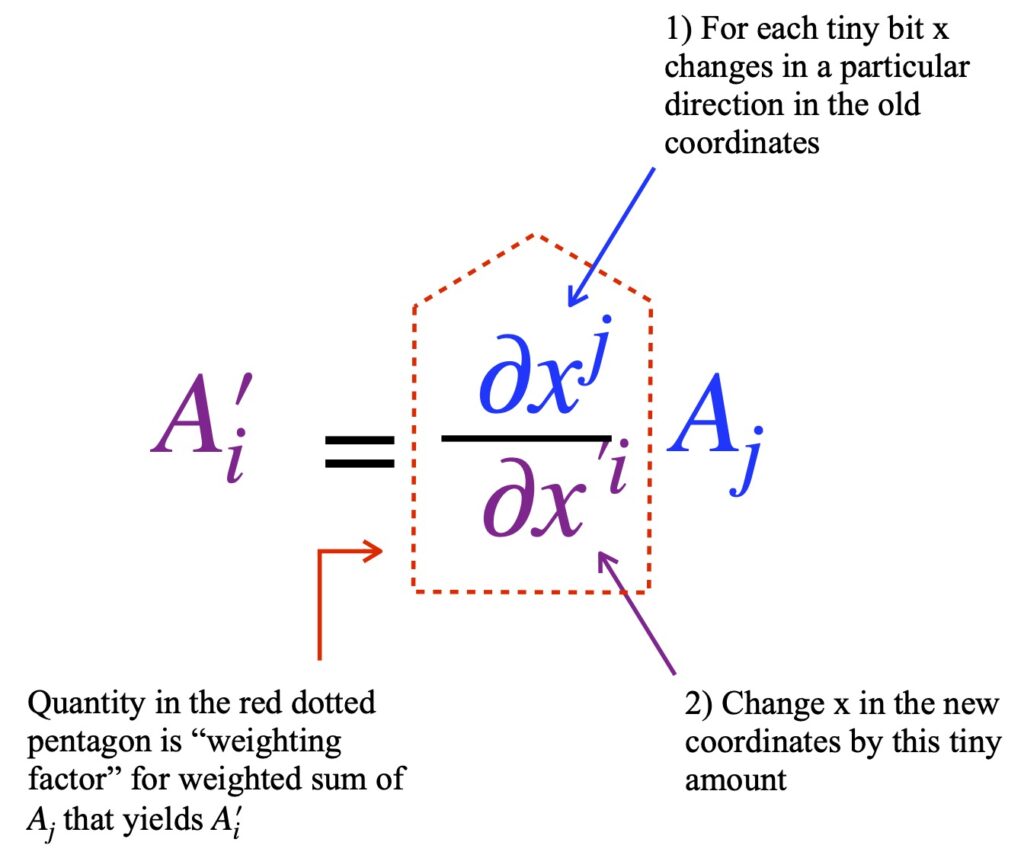
Another way to view the difference between contravariant and covariant components may be even more useful. It’s simply to define the way each type of component changes under coordinate transformations. Contravariant components are said to transform as follows:

Here I’ve used notation I haven’t used before – Einstein summation notation. We’ll also switch from using x, y … as subscripts and superscript to the more commonly-used notation: numbers. Let me explain with an example. For simplicity, we’ll take to be a 3-dimensional vector. In keeping with the way we’ve been transforming vectors, we’ll start by using a transformation matrix:

This matrix equation translates into 3 simultaneous equations:


Of course, this is a lot of writing so mathematicians developed summation notation to make things shorter:


But we still have 3 equations. We can get it down to one equation as follows:

Einstein made the notation even more compact by noting that when there’s a term where an index is used as both a superscript (“upstairs” index) and a subscript (“downstairs” index) – like  is in eq (17) – then one can assume that this index is summed over and the summation sign,
  , can be dropped. Applying Einstein notation to eq (17), we have:

The j in eq (17), the index being summed over, is called a dummy index. That’s because we could replace it with any symbol without changing the meaning of the equation.
The classic example of where contravariant components are used is in transforming the differential length element,  , from one coordinate system to another. Again, we’ll use the commonly-employed convention where
  ,
,  and
and  . We’ll start with a matrix equation:

This matrix equation can be written as 3 simultaneous equations:


As in eq (16), we can reduce eq (20) to 3 summation equations:

We can consolidate the 3 equations of eq (21) into one:

Finally, we can drop the summation sign and wind up with eq (22) in Einstein summation form:

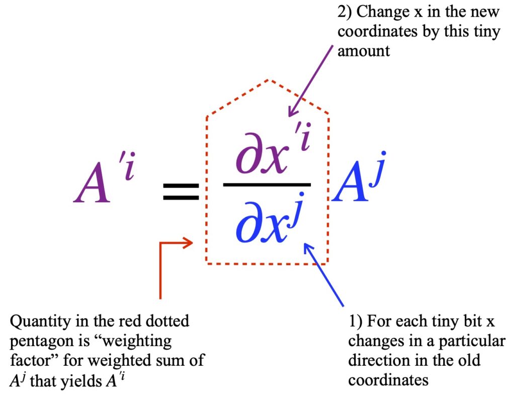
Indeed, many authors define the contravariant components of vector as components that transform as:

Figure II.H.10 is intended to give some intuition regarding how eq (24) might be interpreted.
As you might guess, covariant components can also be defined by the way it transforms under coordinate change. The equation for covariant components is:

where  is a transformation matrix. Notice that whereas superscripts were used for the pre- and post-transformation vectors and subscripts for the transformation matrix with contravariant vector components, the opposite is true for covariant components.
The prototypical example of covariant component use involves the gradient of a scalar field,  (such as room temperature). The change of the field with position is given by the gradient,
  , where again, we use numerical indices instead of x, y, z. Notice that the gradient (per unit length) is the inverse of that of the line element
  which has units of length. We can follow a procedure similar to the one we utilized to derive the contravariant transformation equation for the line element.
First, write a matrix equation:

We write eq (26) as 3 simultaneous equations:


We can write eq (27) as 3 summation equations:
 ,
,  ,
, 
Eq (28) can be reduced to 1 summation equation:

The Einstein summation formula reduces this further to:

In fact, many authors define the covariant components of vector as components that transform as:

The intuition for the meaning of this equation is shown in figure II.H.11:
Having at our fingertips 1) these definitions of contravariant and covariant components given by transformation equations eq (24) and eq (31) and 2) Einstein summation technique, we are now ready to tackle tensors of rank > 1.
III. Tensors of Rank > 1
We spent a significant amount of time talking about vectors because, in this section, we’re going to 1) build rank 2 tensors from vectors and 2) show that the transformation characteristics that define vectors are equally applicable to these rank 2 tensors. Subsequently, we’ll show that higher ranking tensors can be created from lower ranking tensors and follow the same transformation equations. In so doing, this will establish that tensors, in general, are mathematical objects that remain unchanged under coordinate transformations despite changes in components and basis vectors that make them up.
III.A Tensor Creation and Transformations
So how can vectors be used to build rank 2 tensors? By using a vector multiplication method called the outer product. In my mind, the easiest way to visualize the outer product is via matrix multiplication. Specifically:
We start with 2 3-dimensional column vectors
 and
and 
The outer (or tensor) product is defined as:
 eq (32)
In eq (32), the superscript, T, associated with  , is called the transpose. It means make a column a row or vice versa. Once is converted from a column vector to a row vector, it multiplies each component of
  to yield a matrix that represents the rank 2 tensor,
  . Rather than writing
  or
or  , it’s customary to write the tensor product as:
 eq (33)
With its upper indices, it looks like is a contravariant object. Let’s see how transforms under coordinate transformation. We know that is made from and . Thus:
 eq (34)
We know how and transform so:
 eq (35)
 eq (36)
But
 eq (37)
So
 eq (38)
From this, we can say that mathematical objects like  or
or  are tensors – rank 2 tensors with covariant indices.
We can make other types of rank 2 tensors from vectors with other types/combinations of components. Specifically,
 eq (39)
which, by the same arguments presented for eq (33), transforms as
 eq (40)
or
 eq (41)
which transforms as
 eq (42)
or
 eq (43)
which transforms as
 eq (44)
Perhaps you’re beginning to see a pattern.
- If the vectors we use to make the tensor has 2 contravariant indices, then the tensor it creates has the same 2 contravariant indices
- If the vectors we use to make the tensor has 2 covariant indices, then the tensor it creates has the same 2 covariant indices
- If the vectors we use to make the tensor has 1 contravariant and 1 covariant index, then the tensor it creates has the same contravariant and covariant indices
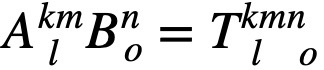
And since we can make a rank 2 tensor out of two rank 1 tensors, as might guess, we can make any higher rank tensor from other lower rank tensors, the higher rank tensor acquiring the indices of the lower rank tensors from which it’s created. For example:
 eq (45)
 eq (46)
And if we wanted to see how such tensors transform, we would simply insert the appropriate partial derivative for each index. For example, the tensor in eq (45) would transform as follows:
 eq (47)
But note that
 eq (48)
To see why, click .


III.B Tensor Properties
III.B.1 Invariance of Tensor Equations
One of the most important properties of tensors is obvious from their transformation properties. Suppose all of the components of a tensor are 0 in one coordinate system. Then by the transformation equations we worked with in the previous section, that tensor must be zero in all coordinate systems:
If  , then the transformed tensor in the new coordinate system,
  must also be 0.
Now suppose  is not 0 but that
 eq (49)
Then
 eq (50)
But we just showed that a tensor that’s 0 in one coordinate system is 0 in all coordinate systems. That means that tensors are invariant and tensor equations are the same in all coordinate systems. The implications of this are critical, especially in physics and engineering, most notably special and general relativity.
III.B.2 Addition and Subtraction
We know we can add vectors (i.e., rank 1 tensors):
 eq (51)
We can do this by adding components:

 eq (52)
We can do something similar with higher ranking tensors:

 eq (53)
To prove that the tensor we created by adding two tensors is itself a tensor, we check to see how it transforms. We’ll use  as an example. It’s made by the addition of
  and . We’ve seen previously seen how and transform:
 eq (54)
and
 eq (55)
So then,  transforms as follows:

 eq (56)
But  . Substituting this into eq (54), we see that transforms like a tensor:
 eq (57)
Thus, the sum of and is another tensor.
We won’t bother to do it here, but I think it’s clear that we could show that the subtraction of a tensor from another is another tensor as well simply be replacing the + sign with a minus sign.
Note that to add or subtract tensors, these tensors have to have the same indices.
III.B.3 Multiplication
We’ve already seen one type of tensor multiplication – the outer product. When we performed the operations that allowed creation of higher ranking tensors from tensors of lower rank, it was the outer product that we used. The mechanics of this procedure is difficult to visualize for higher ranking tensors but we saw how it worked in our discussion of how vectors can be used to make rank 2 tensors.
If you want to see that the outer product of higher ranking tensors transforms like a tensor, click .

 and
and 


 and
and  then
then
Another way to multiply tensors is to take the inner product which we can think of as the generalization of the dot (or scalar) product, which is discussed in the dot product section of my linear algebra page.
When we take the dot product of two vectors, we get a scalar. We can think of the dot product as matrix multiplication:
Let  and
and  . Then the dot product is given by:
 eq (58)
Putting some numbers in, we get:
 eq (59)
So we start with two rank 1 tensors (total “rank” of 2) and end up with a scalar (rank 0).
We also note that  . In Einstein notation,
  . eq (60)
The inner product of a rank 2 tensor with a rank 1 tensor (i.e., vector) can be represented as:
 eq (61)
The Einstein notation for this equation is:
 eq (62)
Notice two things:
- We start with a total rank of 3 (i.e., a rank 2 and a rank 1 tensor) and up with a rank 1 tensor. Thus, like with the dot product of vectors (where the rank went from 2 to 0), the rank, after applying the inner product, is reduces by 2
- When there is a covariant (downstairs) index and a contravariant (upstairs) index in the same expression, then, by Einstein summation convention, that index is summed over, becomes a scalar (i.e., a number) and “disappears” from the expression
This procedure of setting a covariant and contravariant index in the same expression equal to each other, applying the inner product (i.e., summing over that index) and producing a tensor of rank 2 less than the products with which you began is called tensor contraction.
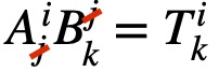
These rules of tensor contraction also apply to higher rank tensors. For example:
 eq (63)
So far, I’ve tried to give some of the theory behind tensors and derive some rules by which they are manipulated. I’ve done this so that, when readers see tensors in action, they will recognize that there are valid reasons for the way they’re being manipulated – that it’s not just magic. However, once established , the most efficient way to work with tensors is simply to apply the rules. Accordingly, at this point, let me summarize a few key points about these rules:
- Tensors are, in part, collections of numbers (components), but what determines these components is the coordinate system in which one is working.
- There are two types of coordinates: contravariant and covariant. Contravariant components are represented with superscripted indices; covariant with subscripted indices.
- The rank of a tensor is given by the number of indices it has.
- Contravariant components are multiplied with superscripted indices to make tensors of rank
 1. Covariant components are multiplied with superscripted indices.
 - Tensors can be multiplied via the outer product to make new tensors. The new tensors inherit the indices of the tensors that are multiplied to make it:
- Tensors can be multiplied via the inner product, a generalization of the vector dot product, to yield a tensor of the original rank – 2. This occurs when the same index occurs as a subscript and superscript in the same expression. In this case, that identical upper and lower index are summed over and dropped from the final expression:
- Tensors with the same indices can be added and subtracted, vector addition and subtraction being the model for how it’s done.
III.C Metric Tensor
III.C.1 Formation
One of the most important tensors in physics is the metric tensor. It’s used to define the geometry of spacetime. Let’s look at how it’s formed.
Consider a vector, . To find its length, we take the dot product with itself:

 eq (64)
Suppose we make very small. As it approaches 0, we’ll call this short length  . If we take its length, what we get is the infinitesimal length element . We find the length of in a manner similar to the way we found vector V’s length; we take the dot product with itself. But we know that:
 eq (65)
Thus,


 eq (66)
where  are the components of the metric tensor. Note that the upstairs indices of the
  and the downstairs indices of the metric tensor create a summation and tensor contraction to a tensor of rank 0 – a scalar (i.e., a number).
For more intuition as to why  is the metric tensor, click .


 eq (66a)
 eq (66b)
 eq (66c)
 eq (66d)


 eq (66e)
 eq (66f)
We can do the same for vectors with covariant component indices:
 eq (67)
Thus,


 eq (68)
When mixed index vectors are used, we have:

 eq (69)
The metric isn’t needed to obtain  in this case because, by the definition of dual basis vectors:
  .
.
In general, the metric helps define the inner product of two tensors (including the dot product of two vectors). And if we define the metric tensor at each point in space, what it does is determine the infinitesimal length element at each point in space, and therefore, the space’s geometry . But more on this in my page on general relativity. For now, let’s start by proving that the metric is indeed a tensor.
III.C.2 Symmetry
We need to show that the metric transforms like the rank 2 tensors we’ve seen so far. Although observers using different coordinate systems won’t agree on the components of an infinitesimal vector  , we know that observers in all coordinates systems will agree on its length . That length is given by:

Now let’s change coordinates. The transformation equation is:
 eq (70)
The transformations for the infinitesimal length vectors go like this:
 eq (71)
Using eq (71) in eq (70), we have:
 eq (72)
For both sides of eq (72) to be equal, the coefficients of  have to be equal. That means that:

So, the metric transforms like a tensor. Therefore, it is a tensor.
Next, let’s look at an important property of the metric: symmetry. The metric tensor is a symmetric tensor. That is,
 ,
,  and
and  eq (70)
For those interested, here’s the :
 eq (1)
 is a symmetric tensor
  eq (2)
 is a antisymmetric tensor
  eq (3)
 eq (4)
 eq (5)
 :
:
 eq (6)
 is a symmetric tensor.
 ?
? . If
. If  is antisymmetric, that means that
 ![N^{ij}=-N^{ji}=-(T^{ij} - T^{ji})^T=[(T^{ji})^T - (T^{ij})^T]=T^{ij} - T^{ji}](https://www.samartigliere.com/wp-content/ql-cache/quicklatex.com-cfe6b1e9094993e4e9897438dd912e5a_l3.png "Rendered by QuickLaTeX.com") which is what we wanted to prove. However, to give you a visual on this like we did with
which is what we wanted to prove. However, to give you a visual on this like we did with 
 eq (7)
 which makes
  and
and  , then
  is a symmetric tensor and
  eq (9)
 is symmetric and
  . Combining this with eq (70a), we get:
 eq (10)
 eq (11)


 eq (12)
III.C.3 Raising and Lowering Indices
Another important application of the metric tensor: raising and lowering indices. It works like this:
We’ve seen previously that:

A metric that multiplies only one vector can be regarded as a covector in that it
- takes in a vector to produce a scalar
- obeys linearity
Call that covector-like entity  . Using this, we can write eq (III.C.3.1) as:

The components of are given by:

We substitute  for
for  in eq (III.C.3.2). We get:
 . Therefore:

In other words, the metric converts the contravariant components of a vector to covariant components i.e., it lowers the contravariant component’s index.
If we start with:

Now multiply both sides by  . We get:

But  , by definition, is the identity matrix. Therefore:
 which means:

In other words, the metric converts the covariant components of a vector to contravariant components i.e., it raises the contravariant component’s index.
As you might expect, since we can make more complex tensors as the tensor product of simple tensors like vectors, we can raise or lower each index of the complex tensor with a separate instance of the metric in appropriate form. Here are some examples:


When we work with such expressions, from a purely mechanistic point of view, we simply apply the following rules:
- Cancel any index that appears as a superscript and subscript in the same expression
- Indices that aren’t cancelled are the indices that remain in the final expression
III.C.4 Examples
In this section, we’ll examine the metric for commonly used coordinate systems, namely polar, cylindrical and spherical coordinates. Therefore, for coordinate systems where axes are orthogonal (like the ones I just mentioned), off-diagonal elements of the metric are zero because, in such cases,  unless
  . Thus, in these cases, to get the metric, we simply put the terms of the line element along the diagonal elements and put zero everywhere else. Fortunately, I’ve derived the line elements for the coordinate systems under consideration elsewhere so the exercise that follows should be simple.
III.C.4.a Polar Coordinates
The line element for polar coordinates is:

Therefore, the metric in polar coordinates is:

III.C.4.b Cylindrical Coordinates
The line element for cylindrical coordinates is:

Therefore, the metric in polar coordinates is:

III.C.4.c Spherical Coordinates
The line element in spherical coordinates is:

Thus, the metric in spherical coordinates looks like this:

IV. Covariant Derivative
IV.A Motivation
Vector fields describe many phenomena in science (e.g., wind speed, fluid movement, the electromagnetic force). We often need to know how these fields are changing at different points in time and space. This is a straightforward process in Euclidean space. One simply takes derivatives of vector components. There’s no need to worry about the basis vectors because, in Euclidean space, they have the same magnitude and direction everywhere. But what happens if the coordinate system we’re using is nonEuclidean i..e., the basis vectors vary from place to place, like spherical coordinates, for example. In that case, we need to take the change in basis vectors, as well as the change in coordinates, into consideration when we take a derivative.
Thus, if we have a 3-dimensional coordinate system where basis vectors  ,
,  and
and  vary at different points, then, for a vector

To obtain the correct derivative, we need to apply the product rule:


This process of accounting for the change in basis vectors when taking a derivative is called covariant differentiation. Of course, since vectors are tensors, and higher rank tensors can be made out of vectors, this process can be generalized to higher rank tensors as well. However, we’ll stick with vectors to illustrate the principles.
The reason we need to take the basis vectors into account when we take the derivative of a tensor is that, if we don’t, we won’t get a tensor back. This creates significant problems for – say physics – where the laws of physics, represented by tensor equations, should be the same in all coordinate systems. For a more in depth illustration of this problem, click .
IV.B Christoffel Symbols
IV.B.1 Definition
The Christoffel symbol is a part of an alternative representation of the righthand-most term in eq (IV.A.3),  :
:

It can be thought of as the component of the vector  . And like other vector components, it can change under coordinate transformations. Therefore, it’ not a tensor. Click on the link for a .
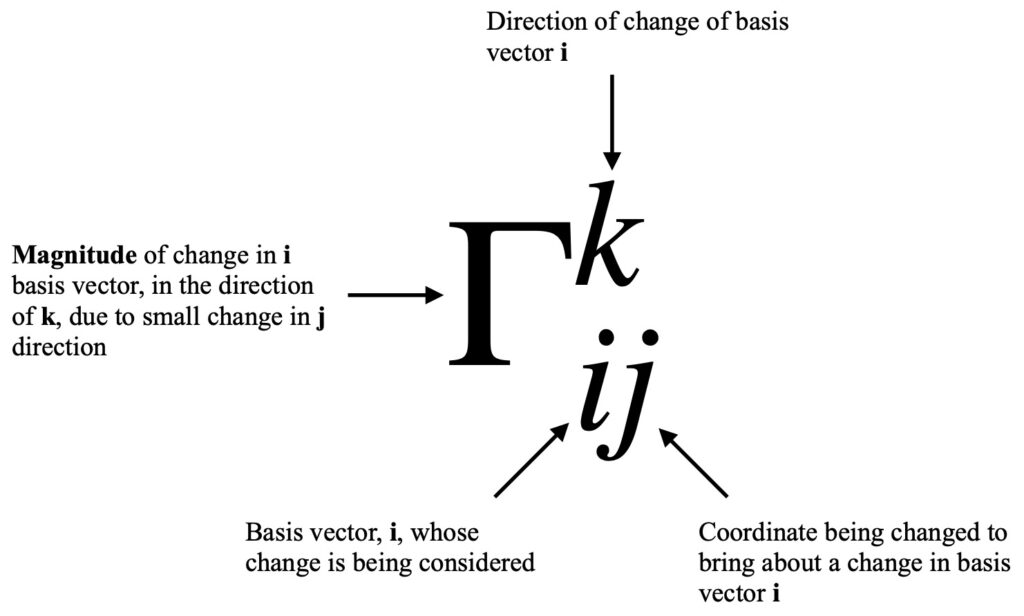
An explanation of what the indices in the Christoffel symbol mean is shown in figure IV.B.1.1.
A useful way to express the Christoffel symbol is in terms of the metric. There are two types of Christoffel symbols:
- Christoffel symbols of the first kind: gives the change in dual basis vectors (i.e., those with a superscript index used to multiply covariant components to make a covector).
- Christoffel symbols of the second kind: gives the change in ordinary basis vectors (i.e., those with a subscript index used to multiply contravariant components to make a vector).
In terms of the metric, Christoffel symbols of the first kind are written as:
![\Gamma_{lij}=\displaystyle \frac12 \left[\displaystyle \frac{\partial g_{li}}{\partial x^j} + \frac{\partial g_{lj}}{\partial x^i} + \frac{\partial g_{ij}}{\partial x^l}\right] \quad \text{eq (IV.B.1.2)}](https://www.samartigliere.com/wp-content/ql-cache/quicklatex.com-267af558275171b7d0c376d3d2ca8ca4_l3.png "Rendered by QuickLaTeX.com")
In terms of the metric, Christoffel symbols of the second kind are written as:
![\Gamma^l_{ij}=\displaystyle \frac12 g^{kl}\left[\frac{\partial g_{ik}}{\partial x^j} + \frac{\partial g_{jk}}{\partial x^i} - \frac{\partial g_{ij}}{\partial x^k}\right] \quad \text{eq (IV.B.1.3)}](https://www.samartigliere.com/wp-content/ql-cache/quicklatex.com-d57ac143310748e8a017922f6583e2fc_l3.png "Rendered by QuickLaTeX.com")
In this article, we’ll concern ourselves mainly with Christoffel symbols of the second kind. Derivations of eq (IV.B.1.3) can be seen by clicking .

 .
.


 , we can write:


 . Use this relationship to substitute for

 and rearrange:
![- \left( \displaystyle \frac{\partial \vec{e}_j}{\partial x^{\,k}} \cdot \vec{e}_i + \displaystyle \frac{\partial \vec{e}_i}{\partial x^{\,k}} \cdot \vec{e}_j \right) \right] \quad \text{(8)}](https://www.samartigliere.com/wp-content/ql-cache/quicklatex.com-855a1f9fb57c9945b5d093d157025be5_l3.png "Rendered by QuickLaTeX.com")


![\Gamma^l_{ij}=\left[ \displaystyle \frac{\partial(\vec{e}_k \cdot \vec{e}_i)}{\partial x^j} + \displaystyle \frac{\partial(\vec{e}_j \cdot \vec{e}_k)}{\partial x^i} - \displaystyle \frac{\partial(\vec{e}_i \cdot \vec{e}_j)}{\partial x^k} \right] \quad \text{(10)}](https://www.samartigliere.com/wp-content/ql-cache/quicklatex.com-13fd3af7bb11b95957fb453ce0fe75e4_l3.png "Rendered by QuickLaTeX.com")
 and
and  , we are left with:
![\Gamma^l_{ij}=\displaystyle \frac12 g^{kl}\left[\frac{\partial g_{ik}}{\partial x^j} + \frac{\partial g_{jk}}{\partial x^i} - \frac{\partial g_{ij}}{\partial x^k}\right] \quad \text{(11)}](https://www.samartigliere.com/wp-content/ql-cache/quicklatex.com-b90694604fc5bd5ef96e238a7610c5a7_l3.png "Rendered by QuickLaTeX.com")


 .
.  is a scalar. Therefore, we can convert the covariant derivative to a regular partial derivative. We have:
 and Clairaut’s theorem, we can convert eq. (14) into:


 and rearranging, we end up with:
IV.B.2 Example
Because of the tedium involved in calculating Christoffel symbols, we’ll take a simple case involving only 2 dimensions, that of polar coordinates.
Because there are 3 indices in Christoffel symbols, the potential number of symbols one might have to calculate is  where
where  is the number of dimensions with which you’re dealing. However, it turns out the Christoffel symbols are symmetric in their lower indices (i.e.,
  . This is because Christoffel symbols are what’s called torsion-free connection coefficients. I won’t explain this here but a conceptual explanation can be found at https://profoundphysics.com/christoffel-symbols-a-complete-guide-with-examples/.
In our case, there are  possible combinations of indices but, because of the symmetry of the lower indices, only 6 independent combinations need to be calculated:


As preparation for performing these calculations, recall the formula for the Christoffel symbol in terms of the metric:
![\[ \Gamma^l_{ij}=\displaystyle \frac12 g^{kl}\left[\frac{\partial g_{ik}}{\partial x^j} + \frac{\partial g_{jk}}{\partial x^i} + \frac{\partial g_{ij}}{\partial x^k}\right] \quad \text{eq (IV.B.1.3)} \]](https://www.samartigliere.com/wp-content/ql-cache/quicklatex.com-0c35aa1c005d906d2ab1086accfebbc3_l3.png "Rendered by QuickLaTeX.com")
Remember also that we are summing over  . Therefore, any term
  where
where  equals zero. We also know that the metric in polar coordinates is

Thus, the only partial derivative that’s nonzero is  .
.
Finally, the inverse metric (that appears in the term  ) is
) is

Considering these facts, we have:
![\Gamma^1_{11}=\displaystyle \frac12 g^{11}\left[\displaystyle \frac{\partial g_{11}}{\partial x^1} + \frac{\partial g_{11}}{\partial x^1} + \frac{\partial g_{11}}{\partial x^1}\right] + \cancel{g^{21}[\dots]}](https://www.samartigliere.com/wp-content/ql-cache/quicklatex.com-3348596388abbbfd6e639e24869e49ef_l3.png "Rendered by QuickLaTeX.com")
![=\,\displaystyle \frac12 (1)\left[ \displaystyle \frac{\partial (1)}{\partial r} + \frac{\partial (1)}{\partial r} - \frac{\partial(1)}{\partial r}\right]](https://www.samartigliere.com/wp-content/ql-cache/quicklatex.com-d4d2d6fc973c62cc9c38f860f8418ab4_l3.png "Rendered by QuickLaTeX.com")

![\Gamma^1_{12}=\displaystyle \frac12 g^{11}\left[\displaystyle \frac{\partial g_{11}}{\partial x^2} + \frac{\partial g_{21}}{\partial x^1} - \frac{\partial g_{12}}{\partial x^1}\right] + \cancel{g^{21}[\dots]}](https://www.samartigliere.com/wp-content/ql-cache/quicklatex.com-11606990cdc56d6d2e0324e793a946d1_l3.png "Rendered by QuickLaTeX.com")
![=\displaystyle \frac12 (1)\left[\displaystyle \frac{\partial (1)}{\partial \theta} + \frac{\partial (0)}{\partial r} - \frac{\partial (0)}{\partial r}\right]](https://www.samartigliere.com/wp-content/ql-cache/quicklatex.com-ed7b4ace7020d8bd3b909f53819481ea_l3.png "Rendered by QuickLaTeX.com")
![\Gamma^1_{22}=\displaystyle \frac12 g^{11}\left[\frac{\partial g_{11}}{\partial x^2} + \frac{\partial g_{21}}{\partial x^1} - \frac{\partial g_{22}}{\partial x^1}\right] + \cancel{g^{21}[\dots]}](https://www.samartigliere.com/wp-content/ql-cache/quicklatex.com-6444a2376e5cc1d918df8f717ca025a3_l3.png "Rendered by QuickLaTeX.com")
![=\displaystyle \frac12 (1)\left[\frac{\partial (1)}{\partial x\theta} + \frac{\partial (0)}{\partial r} - \frac{\partial r^2}{\partial r}\right]](https://www.samartigliere.com/wp-content/ql-cache/quicklatex.com-046f5212a22bb4ec4dddf88b0c82c3a0_l3.png "Rendered by QuickLaTeX.com")
![=\displaystyle (\frac12) \left[0 + 0 - 2r\right]](https://www.samartigliere.com/wp-content/ql-cache/quicklatex.com-de5c9066e418914010ae44f44abe1f1d_l3.png "Rendered by QuickLaTeX.com")

![\Gamma^2_{11}=\cancel{g^{12}[\dots]} + \displaystyle \frac12 g^{22}\left[\frac{\partial g_{12}}{\partial x^1} + \frac{\partial g_{12}}{\partial x^1} - \frac{\partial g_{11}}{\partial x^2}\right]](https://www.samartigliere.com/wp-content/ql-cache/quicklatex.com-2f327e9128ae71fe31618fa546d4f5df_l3.png "Rendered by QuickLaTeX.com")
![=\displaystyle \frac{1}{2r^2}\left[\frac{\partial (0)}{\partial r} + \frac{\partial (0)}{\partial r} - \frac{\partial (1)}{\partial \theta}\right]](https://www.samartigliere.com/wp-content/ql-cache/quicklatex.com-af7955e1b12ecd7b9b40eccf8a809bd2_l3.png "Rendered by QuickLaTeX.com")
![\Gamma^2_{12}=\cancel{g^{12}[\dots]} + \displaystyle \frac12 g^{22}\left[\frac{\partial g_{12}}{\partial x^2} + \frac{\partial g_{22}}{\partial x^1} - \frac{\partial g_{12}}{\partial x^2}\right]](https://www.samartigliere.com/wp-content/ql-cache/quicklatex.com-93ab32aafc348c43e20e705981d70b99_l3.png "Rendered by QuickLaTeX.com")
![=\displaystyle \frac{1}{2r^2}\left[\frac{\partial (0)}{\partial \theta} + \frac{\partial r^2}{\partial r} - \frac{\partial (0)}{\partial \theta}\right]](https://www.samartigliere.com/wp-content/ql-cache/quicklatex.com-22f40ae6c72346ba819f432d60e7a129_l3.png "Rendered by QuickLaTeX.com")
![=\displaystyle \frac{1}{2r^2}\left[ 0+2r+0 \right]](https://www.samartigliere.com/wp-content/ql-cache/quicklatex.com-9741caf4562dbc037fd7b51c92ac7961_l3.png "Rendered by QuickLaTeX.com")

![\Gamma^2_{21}=\cancel{g^{12}[\dots]} + \displaystyle \frac12 g^{22}\left[\frac{\partial g_{22}}{\partial x^1} + \frac{\partial g_{22}}{\partial x^2} - \frac{\partial g_{22}}{\partial x^2}\right]](https://www.samartigliere.com/wp-content/ql-cache/quicklatex.com-b27e31435dc85a4428dbca29de7dacf2_l3.png "Rendered by QuickLaTeX.com")
![=\displaystyle \frac{1}{2r^2}\left[\frac{\partial r^2}{\partial r} + \frac{\partial r^2}{\partial \theta} - \frac{\partial r^2}{\partial \theta}\right]](https://www.samartigliere.com/wp-content/ql-cache/quicklatex.com-a734b5ee368c463909c4b01407a34abc_l3.png "Rendered by QuickLaTeX.com")
![=\displaystyle \frac{1}{2r^2}\left[ 2r + 0 + 0\right]](https://www.samartigliere.com/wp-content/ql-cache/quicklatex.com-59051daef05a08e135b6f558ea3bcd81_l3.png "Rendered by QuickLaTeX.com")
I include this calculation here to show that, indeed,  .
.
![\Gamma^2_{22}=\cancel{g^{12}[\dots]} + \displaystyle \frac12 g^{22}\left[\frac{\partial g_{22}}{\partial x^2} + \frac{\partial g_{22}}{\partial x^2} - \frac{\partial g_{22}}{\partial x^2}\right]](https://www.samartigliere.com/wp-content/ql-cache/quicklatex.com-0518d2949f60ab1d003cbd1b30a47286_l3.png "Rendered by QuickLaTeX.com")
![=\displaystyle \frac{1}{2r^2}\left[\frac{\partial r^2}{\partial \theta} + \frac{\partial r^2}{\partial \theta} + \frac{\partial r^2}{\partial \theta}\right]](https://www.samartigliere.com/wp-content/ql-cache/quicklatex.com-22772384613e5d20893b644e33bbd54d_l3.png "Rendered by QuickLaTeX.com")
![=\displaystyle \frac{1}{2r^2}\left[0+0+0 \right]](https://www.samartigliere.com/wp-content/ql-cache/quicklatex.com-abdbccb2499cb0ea8c2c4180beb356ee_l3.png "Rendered by QuickLaTeX.com")
From these calculations, we can see that only 3 terms are nonzero:


This is typical; in most cases, the majority of terms equal zero. We can also see how laborious even the simplest case is. Normally, such calculations are done by a computer. There is actually a quicker way to do these calculations that involves the Euler-Lagrange equation and the geodesic equation (which we’ll discuss shortly). I won’t go into this method now. However, it is discussed in the reference I alluded to previously: https://profoundphysics.com/christoffel-symbols-a-complete-guide-with-examples
IV.C Covariant Derivative Derivation
Now that we know something about Christoffel symbols, we can move on to deriving the covariant derivative.
We’ve seen how to take the derivative of a vector in non-Cartesian coordinates (where basis vectors are not the same everywhere):

We defined the Christoffel symbol as:

Substituting eq (IV.C.2) into eq (IV.C.1) yields:

 and are dummy indices, and therefore, can be swapped. We have:

We factor out  and get:

The term in parentheses is called the covariant derivative:

It represents the component of the derivative of vector in the direction and – as opposed to Christoffel symbols alone – it is a tensor. Click on the link for a .
Various notations are in use to denote the covariant dervative.  ,
,  ,
,  and
and  are all equivalent expressions.
For covectors we have:

To see why we have a minus sign in this equation, click .
To better see how covariant differentiation works in practice, we can take the example of the covariant derivative of with respect to in polar coordinates:

In this case,  and
and  . Thus we have:

In the previous section on Christoffel symbols, we calculated that:


So


For the second term involving a Christoffel symbol, we have:

So


The complete covariant derivative of with respect to is then:

To apply covariant differentiation to higher rank tensors, on simply adds a Christoffel symbol for each index on the tensor, using a + sign for upper indices and a – sign for lower indices. For example:


IV.D Covariant Derivative of the Metric
Method 1
We can use a method similar to the Leibniz product rule (called metric compatibility) to get a general expression for the covariant derivative of the metric tensor:

So


We change the names of dummy indices so, ultimately, we can factor out a common tensor product:

![=\displaystyle \left[ \frac{g_{rs}}{\partial u^i} - g_{ks} \Gamma^k_{ir} - g_{rk} \Gamma^k_{is} \right] (\epsilon^r \otimes \epsilon^s) \quad \text{eq (IV.D.2)}](https://www.samartigliere.com/wp-content/ql-cache/quicklatex.com-92ea41fd952e043dd0d44ef69593f4ae_l3.png "Rendered by QuickLaTeX.com")
By metric compatibility:

Because  is a scalar, we can convert the covariant derivative to the regular partial derivative. We know that:

Thus, applying metric compatibility, we get:


But, by definition:
 and
and 
Substituting eq (IV.D.6) into eq (IV.D.5), we obtain:


When we put eq (IV.D.7) back into eq (IV.D.2), we’re left with:
![\nabla_{\partial_i}(g) = \displaystyle \left[ \frac{g_{rs}}{\partial u^i} - (\underbrace{g_{ks} \Gamma^k_{ir} + g_{rk} \Gamma^k_{is}}_{\displaystyle \frac{\partial g_{rs}}{\partial u^i}}) \right] (\epsilon^r \otimes \epsilon^s)](https://www.samartigliere.com/wp-content/ql-cache/quicklatex.com-38e8bfdff98bf709d62743cef7fdfc08_l3.png "Rendered by QuickLaTeX.com")


In other words, the covariant derivative of the metric is zero in all directions.
Method 2
From eq. IV.C.15, we know that the covariant derivative of a tensor like the metric is given by:
