Linear Algebra – Sam Artigliere's Blog

Introduction
Vectors
Matrices
Determinants
Eigenvalues and eigenvectors
Diagonalizing a matrix

Introduction

To quote Wikipedia, linear algebra is a branch of mathematics concerning linear equation such as

{\displaystyle a_{1}x_{1}+\cdots +a_{n}x_{n}=b,}

or linear functions such as

{\displaystyle (x_{1},\ldots ,x_{n})\mapsto a_{1}x_{1}+\ldots +a_{n}x_{n},}

and their representations through matrices and vector spaces. (The $\longmapsto$ symbol means the variable on the left maps to the value on the right; I’ll try to stay away from this notation as much as possible).

Vectors

A starting point for linear algebra is a discussion of vectors. Vectors can be defined in number of ways. The most general definition of a vector is that it’s an element of a vector space. A vector space, $V$ , in turn, consists of vectors, a field and 2 operations, discussed below. A field, in general terms, is a commutative ring. However, there’s no reason to go into what a commutative ring is here. Instead, we’ll define a field, $F$ , as the set of real and complex numbers such that adding, subtracting, multiplying or dividing these numbers yields another member of $F$ . The 2 operations alluded to above, more specifically, are

Vector addition is associative: $(u+v)+w=u+(v+w)$ for all $u,v,w \in V$
There is a zero vector, $0$ , such that $u+0=u$ for all $u \in V$
Each vector, $u$ has a negative such that $u-u=o$ for all $u \in V$
Scalar multiplication is associative: $(ab)u=a(bu)$ for any $a,b \ in F$ and $u \in V$
Scalar multiplication is distributive: $(a+b)u=au+bu$ and $a(u+v)=au+av$ for all $a,b \in F$ and $u,v \in V$
Unitarity: There’s an identity element, $I$ such that $Iu=u$ for all $u \in V$

That’s all pretty vague. Here’s a simpler definition that may be more familiar: a vector is an ordered collection of numbers that simultaneously specify a magnitude (represented graphically as length) and direction. The easiest vectors to visualize are vectors in space. The diagram below depicts such vectors.

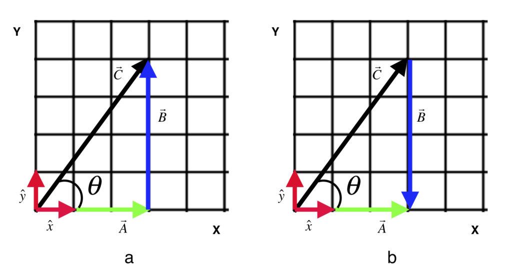
Figure 1 shows three vectors: $\vec A$ , $\vec B$ and $\vec C$ .

Vectors that have the same magnitude (length) and direction represent the same vector, no matter where they’re located in space. For example, $\vec A$ from the figure 1a is the same vector whether its head starts at (0,0) and its tail ends at (0,3) or its head starts at (3,7) and its tail ends at (6,7).
Graphically, we can add vectors together by placing them head to tail. In figure 1a, the head of $\vec B$ is placed at the tail of $\vec A$ to yield $\vec C$ . This is equivalent to the equation $\vec A + \vec B = \vec C$ .
Graphically, we can subtract one vector from another by reversing the direction of the vector to be subtracted and placing its new head at the tail of the vector from which it’s being subtracted. This is depicted in figure 1b and is equivalent to the equation $\vec C - \vec B = \vec A$ .

Vectors can be represented algebraically as a linear combination of unit basis vectors.

Basis vectors are vectors in a vector space, $V$ , such that all other elements of the vector space (i.e., vectors) can be written as a linear combination of these vectors.
Unit basis vectors are basis vectors that are 1 unit in length.
Orthonormal unit basis vectors are unit basis vectors whose dot product (described below) is zero. Orthonormal unit basis vectors are 1 unit in length and are oriented at $90^{\circ}$ to each other. This is true of the Cartesian coordinate system (the usual kind of graph paper you’re used to where axes are at $90^{\circ}$ to each other and units along both axes are equally spaced everywhere). This may not be true when other coordinate systems are used but that’s a discussion for another time. In figure 1, the unit basis vectors are represented by $\hat{x}$ and $\hat{y}$ . (Unit basis vectors, in general, are frequently represented with a little hat over the vector name).
In figure 1, $\vec A$ , can be written as $\vec A = a_x \hat{x} + a_y \hat{y}$ where $a_x$ is called the x-coordinate of $\vec A$ and $a_y$ is called the y-coordinate of $\vec A$ . In the above example, $a_x$ and $a_y$ are scalars (i.e., real or complex numbers). Specifically, $a_x = 3$ and $a_y = 0$ . On the other hand, $\hat{x}$ and $\hat{y}$ are vectors. Their magnitudes are both 1. $\hat{x}$ points in the direction of the x-axis and $\hat{y}$ points along the y-axis.
In figure 1, $\vec B$ , can be written as $\vec B = b_x \hat{x} + b_y \hat{y}$ where $b_x$ is called the x-coordinate of $\vec B$ and $b_y$ is called the y-coordinate of $\vec B$ . As in the case of $\vec A$ , the coordinates of $\vec B$ , $b_x$ and $b_y$ are scalars. Specifically, $b_x = o$ and $b_y = 4$ .
To add vectors A and B, we add the components: $\vec C = \langle a_x + b_x, a_y + b_y \rangle = \langle 3 + 0, 0 + 4 \rangle = \langle 3,4 \rangle = \vec C$ .
This brings up another point: there are several ways that vectors are commonly represented
1. as a bold letter (e.g., $\mathbf {A}$ )
2. with its components in angled brackets, $\langle \, \rangle$ , as we just noted
3. with its components enclosed in brackets; if displayed horizontally, it’s called a row vector (e.g., $\begin{bmatrix} 3&4 \end{bmatrix}$ ); if displayed vertically, it’s called a column vector (e.g., $\begin{bmatrix} 3 \\ 4 \end{bmatrix}$ ). There’s a difference between the two but that difference won’t be of concern for our immediate purposes so we’ll defer discussion about it for now
4. as a point in space, it’s coordinates being the coordinates of the vector
5. as an arrow from the origin of a coordinate system to the point in space corresponding to the vector (as shown above)
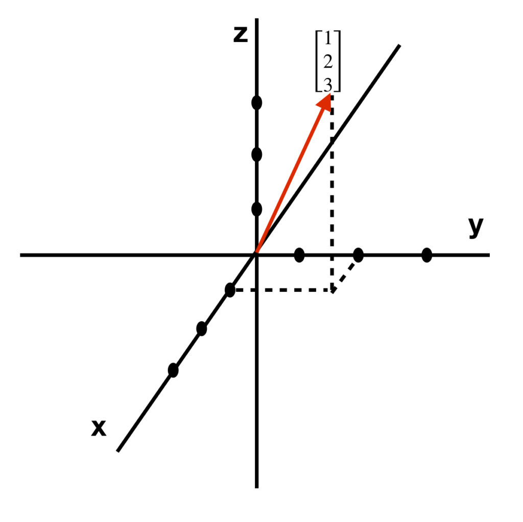
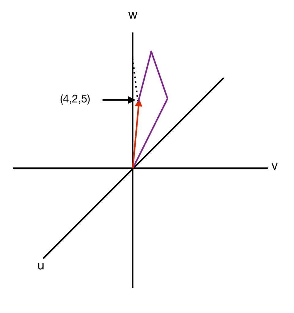
Likewise, to subtract $\vec B$ from $\vec C$ , we subtract components: $\vec C - \vec B = \langle c_x - b_x, c_y - b_y \rangle = \langle 3 - 0, 4 - 4 \rangle = \langle 3,4 \rangle = \vec A$ .

Figure 1 shows an example with 2-dimensional vectors. However, vectors can have as many dimensions as we want. The number of components that the vector contains represents the dimensionality of the vector. For example, $\begin{bmatrix} 1 \\ 2 \\ 3 \end{bmatrix}$ is a 3-dimensional vector that can be depicted graphically as follows:

Linear combinations of vectors

Linear combinations of vectors are combinations of multiplication of vectors by a constant ((i.e., $c$ ) and addition. In the case of 3D vectors, (e.g., $\vec u$ , $\vec v$ , $\vec w$ ):

$c\vec u$ represents a line.

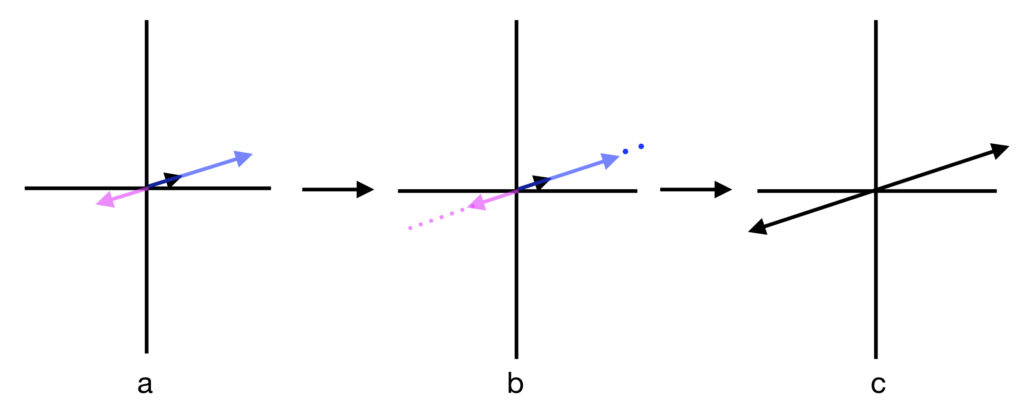
$c \vec u + d \vec v$ fills a plane

$c\vec u + d\vec v + e\vec w$ fills three-dimensional space.

Vector lengths and dot products

Definition:

The dot product or inner product between two vectors $\vec{v}=(v_1,v_2)$ and $\vec{w}=(w_1,w_2)$ is depicted as $\vec{v}\cdot\vec{w}$ and yields a scalar:

$\vec{v}\cdot\vec{w}=v_1w_1+v_2w_2$

Example 1: $\vec{v}=(2,3)$ and $\vec{w}=(2,1)$

$\vec{v}\cdot\vec{w}=v_1w_1+v_2w_2=2\cdot2+3\cdot1=4+3=7$ .

Example 2: $\vec{v}=(4,2)$ and $\vec{w}$ =(-1,2)

$\vec{v}\cdot\vec{w}=v_1w_1+v_2w_2=4\cdot-1+2\cdot2=-4+4=0$ .

Note that if the dot product of two vectors equals zero, the two vectors are said to be orthogonal. If we’re talking about 2D and 3D vectors in the usual Cartesian coordinate system that we’re used to, orthogonal means that they are perpendicular (i.e., the angle between them is $90^\circ$ ).

If we’re dealing with 3D vectors like $\vec{v}=(v_1,v_2,v_3)$ and $\vec{w}=(w_1,w_2,w_3)$ then the dot product is

$\vec{v}\cdot\vec{w}=v_1w_1+v_2w_2+v_3w_3$

For higher dimensional vectors (e.g. n-dimensional vectors $\vec{v}=(v_1,v_2,\dots,v_n)$ and $\vec{w}=(w_1,w_2,\dots,w_n)$ , the dot product is:

$\vec{v}\cdot\vec{w}=v_1w_1+v_2w_2+\dots+v_nw_n=\displaystyle\sum_{i=1}^n v_i w_i$

Dot product properities

Consider a scalar, $c$ and three vectors, $\vec{v}$ , $\vec{w}$ and $\vec{z}$ . The dot product for these vectors has the following properties:

- Commutativity: $\vec{v}\cdot\vec{w}=\vec{w}\cdot\vec{v}$
- Distributivity with addition: $\vec{z}(\vec{v}+\vec{w})=\vec{z}\vec{v}+\vec{z}\vec{w}$
- Distributivity with multiplication: $c(\vec{v}\cdot\vec{w})=(c\vec{v})\cdot\vec{w})$

The proofs for these properties lie, basically, in computing the value of each side of each of the above equations and are quite tedious. Therefore, they will be left to the reader. However, examples of proofs of some of these properties can be found here (Khan Academy).

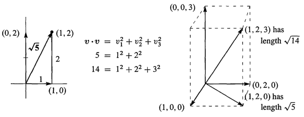
Vector lengths

The length of a vector $\lvert \vec{v} \rvert$ of a vector is the square root of $\vec{v}\cdot\vec{v}$ :

$\text{length}=\lvert \vec{v} \rvert=\sqrt{\vec{v}\cdot\vec{v}}$

In two dimennsions, length is $\sqrt{v_1^2+v_2^2}$ . In three dimensions, it is $\sqrt{v_1^2+v_2^2+v_3^2}$ . In four dimensions, it’s $\sqrt{v_1^2+v_2^2+v_3^2+v_4^2}$ , and so on. In these formulas, the subscripts represent components of the vector $\vec{v}$ . This is just a statement of the Pythagorean theorem. A proof of why this is so can be found here.

Here are two examples taken directly from Strang’s textbook, p. 13:

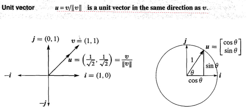
Unit vectors

A unit vector is a vector that is one unit in length.

To find the components of a unit vector in the direction of any vector, $\vec{v}$ , divide the component, $v_i$ by the length of the vector, $\displaystyle \lvert v \rvert$ .
Unit vectors along the x and y axis of the Cartesian coordinate system that we’re used to are commonly denoted $\hat{i}=(1,0)$ (for the x-axis) and $\hat{j}=(0,1)$ (for the y-axis).
The components of a unit vector that makes an angle $\theta$ with the x-axis is $(\cos {\theta},\sin{\theta})$ .

Here are examples taken from Strang’s textbook, p. 13:

Dot product formula using cosine

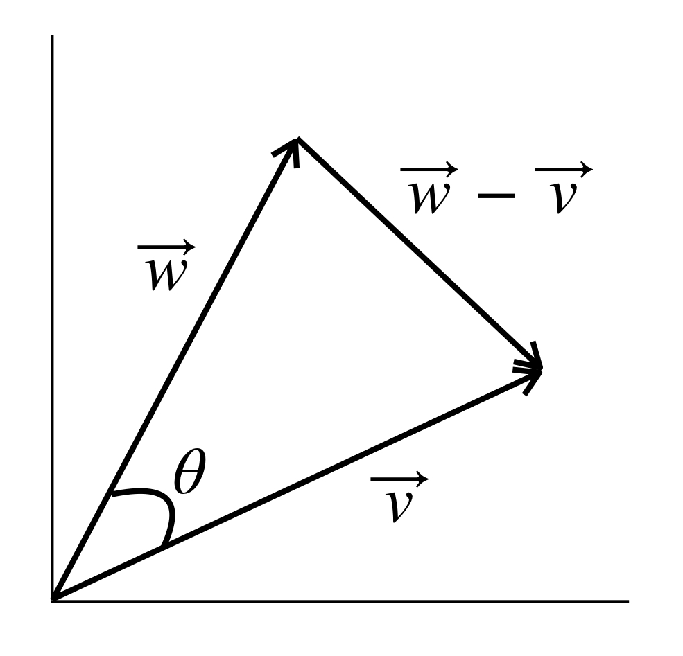
Referring to the diagram above, the law of cosines tells us that:

$\lvert \vec{v}-\vec{w} \rvert^2=\lvert \vec{v} \rvert^2+\lvert \vec{w} \rvert^2-2\lvert \vec{v} \rvert \lvert \vec{w} \rvert \cos{\theta}$

Using dot product properties, we can write the left-hand side of this equation as:

$\begin{array}{rcl}\lvert \vec{v}-\vec{w} \rvert^2 &=& (\vec{v}-\vec{w})\cdot(\vec{v}-\vec{w}) \\ &=& \vec{v}\cdot\vec{v} - \vec{v} \cdot \vec{w} - \vec{w} \cdot \vec{v} + \vec{w}\cdot\vec{w} \\ &=& \lvert \vec{v} \rvert^2 - 2\vec{v} \cdot \vec{w} + \lvert \vec{w} \rvert^2 \end{array}$

Substituting this into our original equation, we get:

$\lvert \vec{v} \rvert^2 - 2\vec{v} \cdot \vec{w} + \lvert \vec{w} \rvert^2=\lvert \vec{v} \rvert^2+\lvert \vec{w} \rvert^2-2\lvert \vec{v} \rvert \lvert \vec{w} \rvert \cos{\theta}$

Now subtract $\lvert \vec{v} \rvert^2$ and $\lvert \vec{w} \rvert^2$ from both sides of the equation. We have:

$- 2\vec{v} \cdot \vec{w}=-2\lvert \vec{v} \rvert \lvert \vec{w} \rvert \cos{\theta}$

Divide both sides of the equation by $-2$ . We are left with:

$\vec{v} \cdot \vec{w}=\lvert \vec{v} \rvert \lvert \vec{w} \rvert \cos{\theta}$

and

$\cos{\theta}=\frac{\vec{v} \cdot \vec{w}}{\lvert \vec{v} \rvert \lvert \vec{w} \rvert}$

Two important inequalities

There are two important inequalities that are a direct consequence of the dot product. They are:

Schwarz inequality: $\lvert \vec{v}\cdot\vec{w}\rvert\leq\lvert \vec{v} \rvert\cdot\lvert \vec{w} \rvert$
Triangle inequality: $\lvert \vec{v}+\vec{w}\rvert\leq\lvert \vec{v} \rvert+\lvert \vec{w} \rvert$

Proofs of these inequalities can be found at http://people.sju.edu/~pklingsb/cs.triang.pdf

Linear equations

Ultimately, linear algebra is about solving linear equations, especially systems of linear equations (i.e., multiple simultaneous linear equations). We call such equations linear equations because they can be represented as linear combinations of vectors. Here is a simple example borrowed from Dr. Gilbert Strang¹

$\begin{align*}2x-y &= 1 \\ x + y &=5\end{align*}$

This set of equations can be looked at in two ways:

Row picture

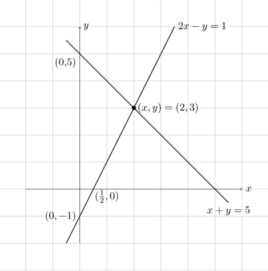
The equations $2x-y=1$ and $x+y=5$ , which extend left to right across the page (like a row in a table) each represent a line. (To see why this is so, check out this review.) The point where the 2 lines intersect, $(x,y)=(2,3)$ represents the solution to the system of equations.

We can show that this is true algebraically. Start by adding equation 1 to equation 2:

$\begin{align*} 2x-y &= 1 \quad \,\,\text{eq. 1}\\+\,\,\+(x+y&=5) \quad \text{eq. 2}\\ \cline{1-2} 3x &= 6 \\ x &= 2\end{align*}$

Back substitute $x=2$ into equation 2:

$\begin{align*} 2+y &= 5 \\ y&= 3\end{align*}$

So $x=2$ and $y=3$ .

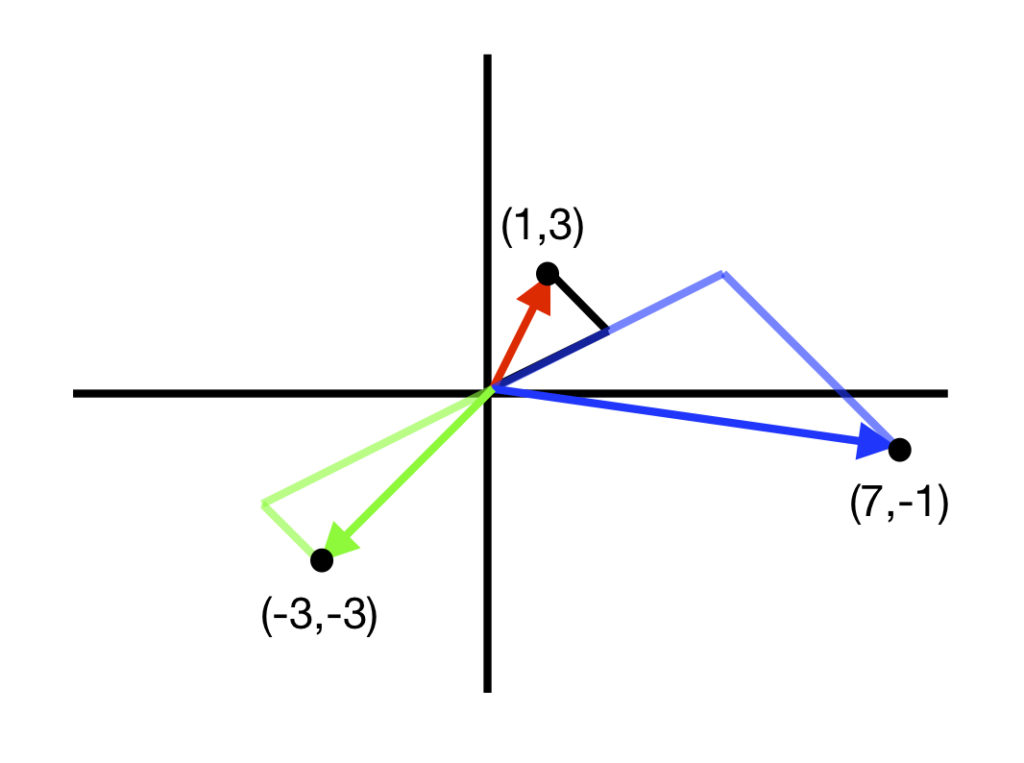
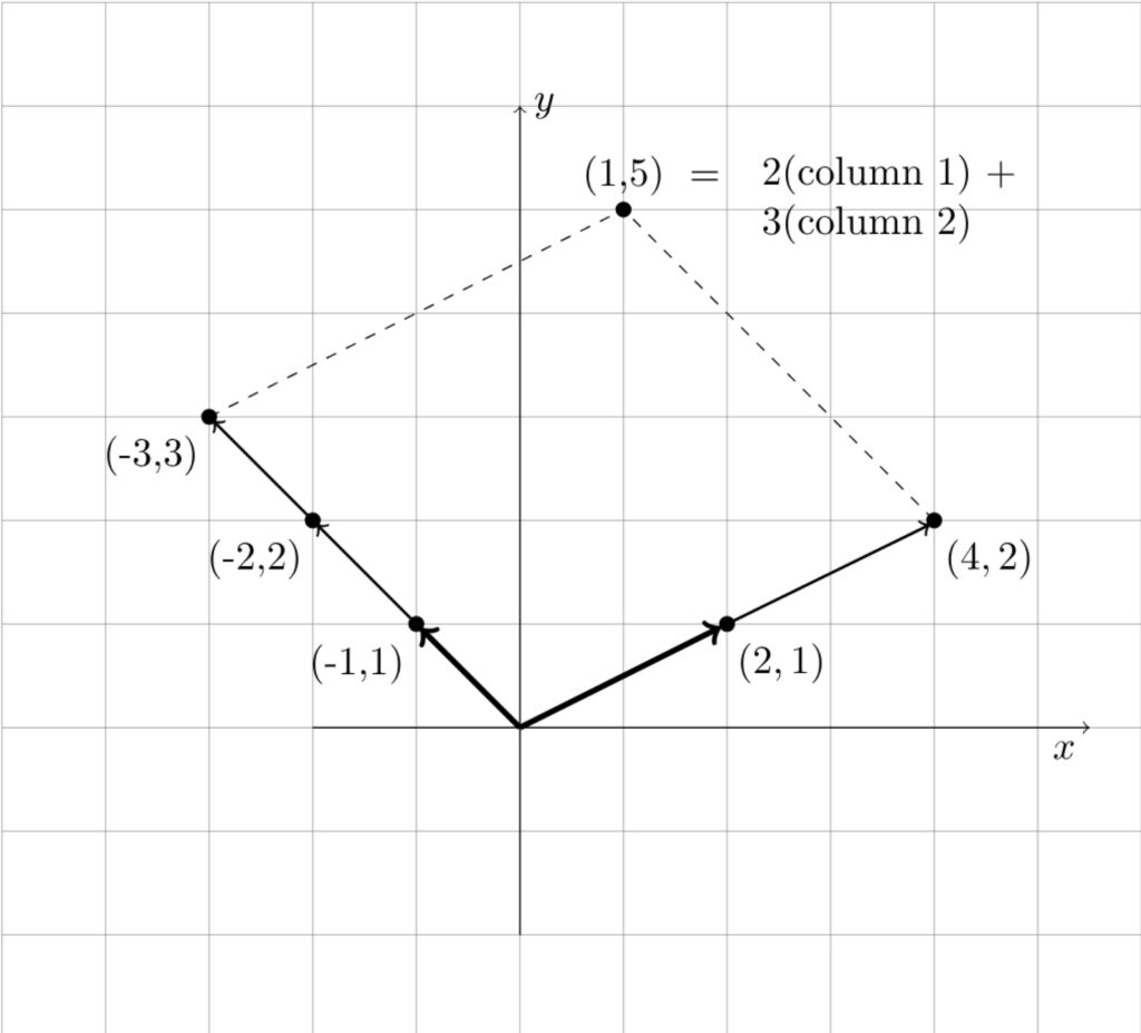
Column picture

Look at our system of equations:

$\begin{align*}2x-y &= 1 \\ x + y &=5\end{align*}$

This can be rewritten as

$\begin{bmatrix} 2x\\x \end{bmatrix} + \begin{bmatrix} -y\\\,\,\,\,\,y \end{bmatrix} = \begin{bmatrix} 1\\5 \end{bmatrix}$

Factor out $x$ and $y$ :

$x\begin{bmatrix} 2\\1 \end{bmatrix} + y\begin{bmatrix} -1\\\,\,\,\,\,1 \end{bmatrix} = \begin{bmatrix} 1\\5 \end{bmatrix}$

Note that $\begin{bmatrix} 2\\1 \end{bmatrix}$ and $\begin{bmatrix} -1\\\,\,\,\,\,1 \end{bmatrix}$ are column vectors. Thus, to solve this equation, we need to find values of $x$ and $y$ that produce a linear combination (or combinations) that yield the column vector $\begin{bmatrix} 1\\5 \end{bmatrix}$ . As you might guess, those values are $x=2$ and $y=3$ . The following diagram illustrates that this is so.

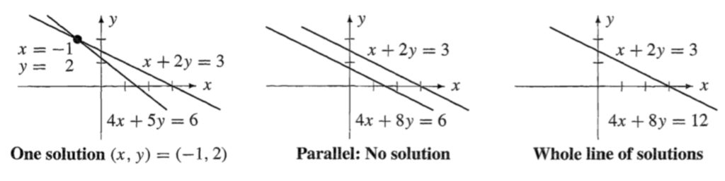
Solutions to linear equations

In the example above, there was one solution to the system of equations being considered. However, when attempting to solve a system of linear equations, there are 3 possible outcomes (seen best when considering the row view):

One unique solution (line’s intersect)
No solution (lines are parallel)
An infinite number of solutions (lines overlap)

The following diagram taken from Strang’s texbook may make this clearer:

The situation is similar for systems of 3 linear equations. An example, again taken from Strang, will help to illustrate this:

$\begin{align*} 2x+y+z &= \, \, \, \, 5 \quad \text{eq. 1} \\ 4x-6y &=-2 \quad \text{eq. 2} \\ -2x+7y+2z &= \, \, \, \, 9 \quad \text{eq. 3} \end{align*}$

The solution to this system of equations is $x=1$ , $y=1$ and $z=2$ .

All of the linear combinations that can be made from each of the equations in the example above yields a plane in 3D space. Like in the 2D case, there are 3 types of possible solutions:

if the planes intersect at a point, then there is one unique solution to the system of equations
if all 3 planes do not intersect, then there is no solution
if the intersection of the 3 planes form a line, then there are an infinite number of solutions

When plotted using a free online graphing program,

https://technology.cpm.org/general/3dgraph/

the planes formed by the system of equations in our 3D example look like this:

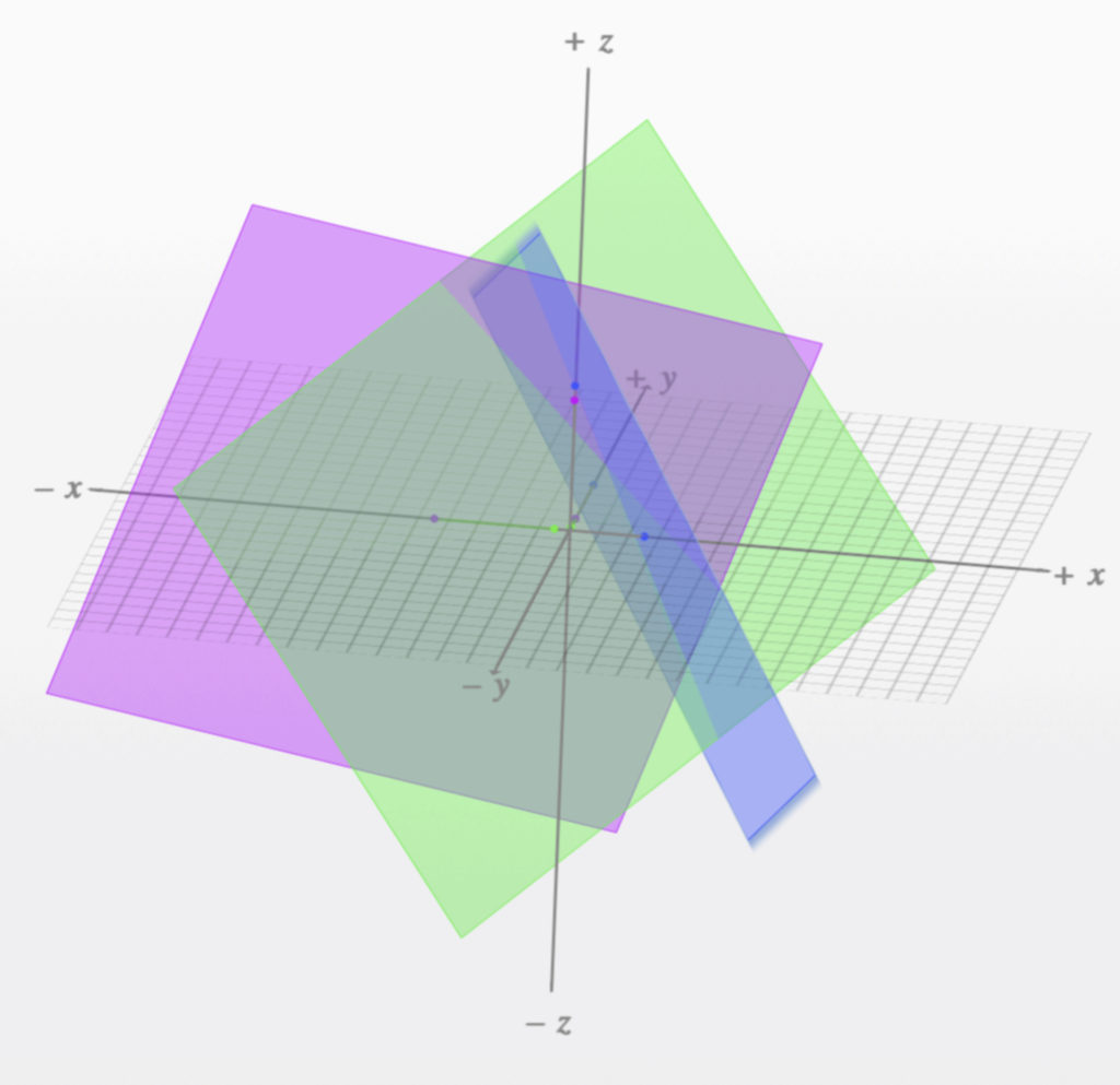
We can see from the diagram that the three planes intersect at a point. It’s difficult to precisely define this point on the diagram because of the difficulty in angling the axes in a way that optimally visualizes all three coordinates at once. However, if we could, the point that we would define would be $(1,1,2)$ .

Matrices

A more efficient way to solve systems of linear equations is to make use of matrices. We’ll use the systems of equations we’ve considered above to illustrate how this works.

The general formula we’ll use is $A\vec x=\vec b$ where $A$ is a matrix, $x$ is a vector and $b$ is another vector. In the 2D example,

Take the coefficients on the left side of the system of equations and place them inside brackets, maintaining their row/column structure: $\begin{bmatrix} 2 & -1 \\ 1 & \,\,\,\,\,1 \end{bmatrix}$ . This is the matrix $A$ .
Place the variables, $x$ and $y$ , into a column, $\begin{bmatrix} x \\ y \end{bmatrix}$ . This is the vector $\vec x$ .
Place the numbers on the right side of the equations into a column $\begin{bmatrix} 1 \\ 5 \end{bmatrix}$ . This is the vector $\vec b$ .

This gives us

$\begin{equation*}\begin{bmatrix} 2 & -1 \\ 1 & \,\,\,\,\,1 \end{bmatrix} \begin{bmatrix} x \\ y \end{bmatrix} = \begin{bmatrix} 1 \\ 5 \end{bmatrix} \end{equation*}$

To get back to our original system of linear equations, we need to apply matrix multiplication.

Mechanics of matrix multiplication

Matrix times a vector

2D matrix multiplication with a vector

Multiplying a matrix times a vector ( $A\vec x$ ) involves taking the dot product of the vector, $x$ with each of the columns of $A$ to create a new “1-column matrix” (better known as a vector). To illustrate this, let’s consider the simple 2D example first:

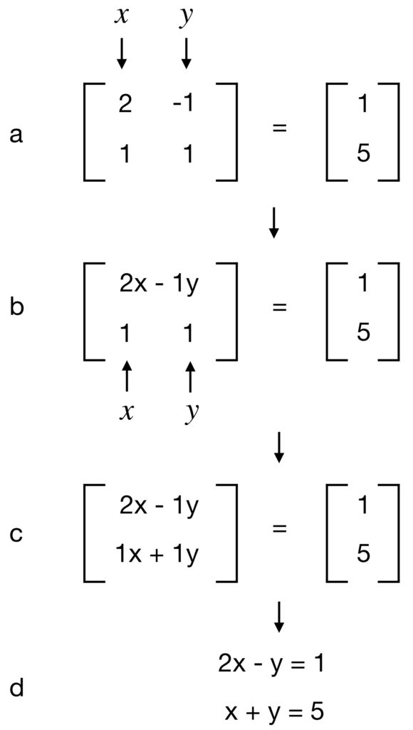
a – Take the dot product of $\vec x$ with the first row of the matrix by multiplying $x$ times $2$ and adding that to the product of $y$ times $1$ . Then place that sum as a single entry in the top row of the matrix to yield the results seen in b.
b – Take the dot product of $\vec x$ with the second row of the matrix by multiplying $x$ times $1$ and adding that to the product of $y$ times $1$ . Then place that sum as a single entry in the top row of the matrix to yield the results seen in c.
c – Split the matrices into separate equations as in d.
d – We have 2 equations in 2 rows, which is just what we started with.
This shows that such a system of equations (i.e., the row description of these equations) is equivalent to our matrix equation.

Finally, we can take our matrix, and instead of taking the dot product of each row, we can multiply each column of our matrix by the appropriate coefficient of the vector (in this case, $x$ for our first column and $y$ for our second column). This gives us the column representation of our system of equations:

$x\begin{bmatrix} 2\\1 \end{bmatrix} + y\begin{bmatrix} -1\\\,\,\,\,\,1 \end{bmatrix} = \begin{bmatrix} 1\\5 \end{bmatrix}$

3D matrix multiplication with a vector

The 3-dimensional case is a bit more rigorous but follows the same principles. To illustrate this, we’ll examine the 3D system of equations we considered previously:

$\begin{align*} 2u+v+w &= \,\,\,\,\,5 \\ 4u-6v &=-2 \\ -2u+7v+2w &= \,\,\,\,\,9 \end{align*}$

As we’ve seen, this system of equations can be represented as follows:

$\begin{equation*}\begin{bmatrix} \,\,\,\,\,2 & \,\,\,\,\,1 & 1 \\ \,\,\,\,\,4 & -6 & 0 \\ -2 & \,\,\,\,\,7 & 2 \end{bmatrix}\begin{bmatrix} u \\ v \\ w\end{bmatrix}=\begin{bmatrix} \,\,\,\,\,5 \\ -2 \\ \,\,\,\,\,9\end{bmatrix}\text{note that () can be used instead of [ ]}\end{equation*}$

We can move back to our original system of 3 equations by using matrix multiplication:

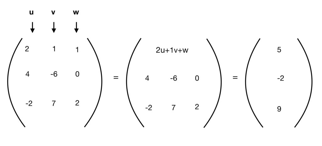
Step 1: Multiply the top row of the matrix by the column vector $\begin{pmatrix} u \\ v \\ w\end{pmatrix}$ (i.e., multiply $u$ times $2$ , $v$ times $1$ and $w$ times 1). Add these products together and make this sum the first row/first column in a new matrix.

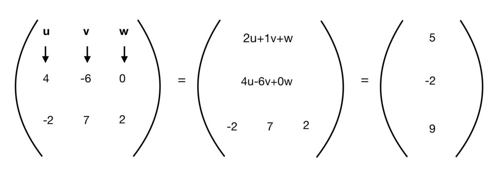
Step 2: Multiply the second row of the matrix by the column vector $\begin{pmatrix} u \\ v \\ w\end{pmatrix}$ (i.e., multiply $u$ times $4$ , $v$ times $-6$ and $w$ times 0). Add these products together and make this sum the second row/first column in the new matrix.

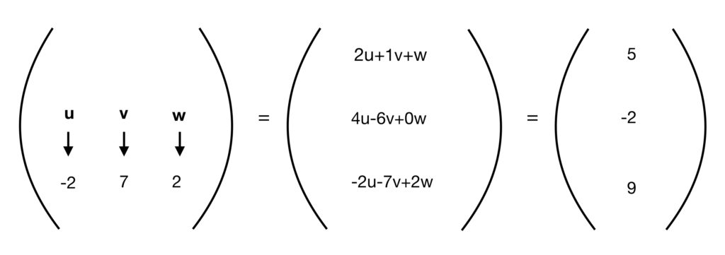
Step 3: Multiply the top third row of the matrix by the column vector $\begin{pmatrix} u \\ v \\ w\end{pmatrix}$ (i.e., multiply $u$ times $-2$ , $v$ times $7$ and $w$ times 2). Add these products together and make this sum the third row/first column in a new matrix.

With this, we’re back to our original system of equations, represented in row form. Of course, if we multiply each column by the appropriate vector coefficient (i.e., $u$ for the first column, $v$ for the first column and $w$ for the first column, we get the also-equivalent column representation:

$u \begin{bmatrix} \,\,\,\,\,2\\\,\,\,\,\,4\\-2\end{bmatrix}+v\begin{bmatrix} \,\,\,\,\,1\\-6\\\,\,\,\,\,7\end{bmatrix}+w\begin{bmatrix} 1\\0\\2\end{bmatrix}=\begin{bmatrix} \,\,\,\,\,5\\-2\\\,\,\,\,\,9\end{bmatrix}$

Matrix times matrix

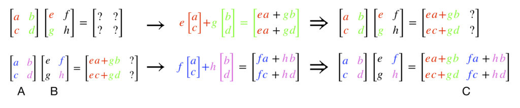
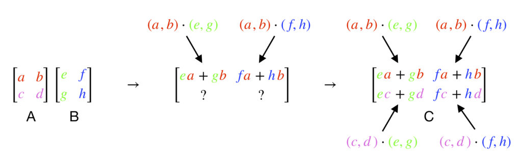
We can also multiply 2 matrices, $A$ and $B$ together to get a new matrix, $C$ . To do this, the dot product of each column in the matrix on the right of a matrix-matrix multiplication expression is taken with the rows of the matrix on the left, exactly like in matrix-vector multiplication. This creates a column in a new matrix with a relative position that is the same as the column that was used to create it. It looks like this:

$\begin{bmatrix} a_{11} & a_{12} &a_{13} \\ a_{21} & a_{22} &a_{23} \\ a_{31} & a_{32} &a_{33} \end{bmatrix}\begin{bmatrix} b_{11} & b_{12} & b_{13} \\ b_{21} & b_{22} & b_{23} \\ b_{31} & b_{32} & b_{33} \end{bmatrix}=$

$\begin{bmatrix} a_{11}b_{11} + a_{12}b_{21} + a_{13}b_{31} & a_{11}b_{12} + a_{12}b_{22} + a_{13}b_{32} & a_{11}b_{13} + a_{12}b_{23} + a_{13}b_{33} \\ a_{21}b_{11} + a_{22}b_{21} + a_{23}b_{31} & a_{21}b_{12} + a_{22}b_{22} + a_{23}b_{32} & a_{21}b_{13} + a_{22}b_{23} + a_{23}b_{33} \\ a_{31}b_{13} + a_{32}b_{23} + a_{33}b_{33} & a_{31}b_{13} + a_{32}b_{23} + a_{33}b_{33} & a_{31}b_{13} + a_{32}b_{23} + a_{33}b_{33} \end{bmatrix}$

An example with numbers is as follows:

$\begin{bmatrix} 1 & \,\,\,\,\,0 & 4 \\ 3 & -1 & 2 \\ 0 & \,\,\,\,\,3 & 1 \end{bmatrix}\begin{bmatrix} \,\,\,\,\,2 & \,\,\,\,\,1 & 1 \\ -2 & \,\,\,\,\,3 & 1 \\ \,\,\,\,\,1 & -1 & 4 \end{bmatrix}=\begin{bmatrix} \,\,\,\,\,6 & -3 & 17 \\ \,\,\,\,\,10 & -2 & 10 \\ -5 & \,\,\,\,\,8 & 7 \end{bmatrix}$

The identity matrix, I

The identity matrix is a matrix with 1’s on its diagonal elements and 0’s everywhere else. For example

Examples

$I \,=\, \begin{bmatrix} 1 & 0 \\ 0 & 1 \end{bmatrix} \,=\, \begin{bmatrix} 1 & 0 & \dots & 0 & 0\\ 0 & 1 & \dots & 0 & 0\\ \vdots & \vdots & \ddots & \vdots & \vdots\\ 0 & 0 & \dots & 1 & 0\\ 0 & 0 & \dots & 0 & 1\end{bmatrix}$

Properties

1. Any matrix multiplied by the identity matrix gives back the original matrix

$AI=A\quad \text{and}\quad IA=A$

For example

$\begin{bmatrix}2&1\\1&3\end{bmatrix}\begin{bmatrix}1&0\\0&1\end{bmatrix}=\begin{bmatrix}2&1\\1&3\end{bmatrix} \quad \text{and} \quad \begin{bmatrix}1&0\\0&1\end{bmatrix}\begin{bmatrix}2&1\\1&3\end{bmatrix}=\begin{bmatrix}2&1\\1&3\end{bmatrix}$

Geometric interpretation of matrix multiplication

As suggested in our previous discussion related to systems of linear equations, an evaluation of the geometry of matrix multiplication may further our understanding of the process. Specifically, it may be helpful to think of the matrix as a machine that performs an operation on a vector to yield a new vector. The operation it performs is a linear transformation. Geometrically, what this means is that the matrix establishes the coordinate system in which the vector should be represented.

It’s useful to realize that the matrix equation $A\vec x = \vec b$ is equivalent to the equation $A\vec x = I\vec b$ where $I$ is the identity matrix. This viewpoint is because 1) the identity matrix times any matrix gives back the original matrix and 2) a vector can be thought of as a one dimensional matrix. It turns out that the coordinate system that $I$ creates is just the Cartesian coordinate system with which we’re all familiar where 1) the basis vectors used to build up other vectors are unit vectors perpendicular to each other 2) the axes of the coordinate system are perpendicular to each other and 3) the spacing between units on those axes is 1 unit in length everywhere.

What the linear transformation performed by $A$ does is change the length and direction of basis vectors from that created by $I$ while 1) keeping the origin of the coordinate system at the same point as the Cartesian coordinate system and 2) keeping grid lines associated with the coordinate system straight, parallel and evenly spaced.

What solving a matrix equation like $A\vec x = \vec b$ ultimately involves, then, is finding the coordinates of $\vec x$ , in the coordinate system created by $A$ , that make the end of the vector so created land on the same point in space as that specified by the vector $\vec b$ in the coordinate system created by $I$ . In essence, the vectors on both sides of the matrix equation point to the same point in space. It’s just that we are “looking at space” differently in the two coordinate systems. This is what makes the coefficients of $\vec x$ and $\vec b$ different.

2D example

I realize that these ideas, as expressed in words in the previous paragraphs, seem convoluted. Therefore, let me try to make things clearer with an example. Let’s consider the 2D system of equations we’ve been working with already:

$\begin{align*}2x-y &= 1 \\ x + y &=5\end{align*}$

The matrix equation that corresponds to this system of equations is:

$\begin{bmatrix} 2 & -1 \\ 1 & \,\,\,\,\,1 \end{bmatrix}\begin{bmatrix} x \\ y \end{bmatrix} = \begin{bmatrix} 1 \\ 5 \end{bmatrix}$

This is equivalent to:

$\begin{bmatrix} 2 & -1 \\ 1 &\,\,\,\,\, 1 \end{bmatrix}\begin{bmatrix} x \\ y \end{bmatrix} = \begin{bmatrix} 1 & 0\\ 0 & 1 \end{bmatrix}\begin{bmatrix} 1 \\ 5 \end{bmatrix}$

The column picture of this equation is:

$x\begin{bmatrix} 2\\1 \end{bmatrix} + y\begin{bmatrix} -1\\\,\,\,\,\,1 \end{bmatrix} = \begin{bmatrix} 1\\5 \end{bmatrix}$

This is equivalent to:

$x\begin{bmatrix} 2\\1 \end{bmatrix} + y\begin{bmatrix} -1\\\,\,\,\,\,1 \end{bmatrix} = 1\begin{bmatrix} 1\\0 \end{bmatrix} + 5\begin{bmatrix} 0\\1 \end{bmatrix}$

To solve this equation, in this simple example, a picture will help:

In the diagram:

The thick black lines represent the x (horizontal) and y (vertical) axes of the Cartesian coordinate system created by $I$
The grid of light blue lines represents the coordinate grid of that Cartesian coordinate system
The thick blue lines represent the x and y axes of the coordinates system specified by matrix $A$
The darker blue lines that are parallel to the thick blue axes represent the coordinate grid associated with matrix $A$

If we let $\hat{i}$ represent the unit vector in the x-direction of the Cartesian coordinate system and $\hat{j}$ represent the unit vector in the y-direction. Then,

Matrix $A$ transforms $\hat{i}=\begin{bmatrix} 1 & 0 \end{bmatrix}$ to $\hat{i^\prime}=\begin{bmatrix} 2 & 1 \end{bmatrix}$
Matrix $A$ transforms $\hat{j}=\begin{bmatrix} 0 & 1 \end{bmatrix}$ to $\hat{j^\prime}=\begin{bmatrix} -1 & 1 \end{bmatrix}$
Note that the columns of our matrix, $A$ , are the new basis vectors that our matrix creates: the left-hand column is the transformed version of $\hat{i}$ (which we’re calling $\hat{i^\prime}$ ; the right-hand column is the transformed version of $\hat{j}$ (which we’re calling $\hat{j^\prime}$ )

The green lines represent the vector addition in the Cartesian coordinate system:

+1 unit in the direction of $\hat{i}$
+5 units in the direction of $\hat{j}$

The red lines represent the vector addition needed to get to the same point in space in the coordinate system specified by $A$ . That vector addition is:

$x=+2$ units in the direction of $\hat{i^\prime}$
$y=+3$ units in the direction of $\hat{j^\prime}$

The above discussion is based on the following YouTube video from 3Blue1Brown: https://www.youtube.com/watch?v=kYB8IZa5AuE

I encourage readers to watch the entire series because 1) it explains the “why” behind a multitude of concepts, something that is missing in many discussions on linear algebra and 2) it has some great animations that illustrate these concepts more clearly than words and equations ever could.

3D and higher dimensional linear transformations

As you might guess, we can apply this linear transformation perspective to 3D equations in a manner similar to the way it was applied to the 2D situation. The 3D equation system we’ve examined previously will serve as an illustration. Recall that the column view of that system was expressed as follows:

We can use this equation to make a matrix equation of the form $A\vec x = \vec b$ :

$\begin{bmatrix} \,\,\,\,\,2&\,\,\,\,\,1&\,\,\,\,\,1 \\ \,\,\,\,\,4&-6&\,\,\,\,\,0 \\ -2&\,\,\,\,\,7&\,\,\,\,\,2\end{bmatrix}\begin{bmatrix} u\\v\\w\end{bmatrix} = \begin{bmatrix} \,\,\,\,\,5\\-2\\\,\,\,\,\,9\end{bmatrix}$

The basis vectors that we’ll use to produce the Cartesian coordinate system and define the 3D vector, $\begin{bmatrix} \,\,\,\,\,5\\-2\\\,\,\,\,\,9\end{bmatrix}$ are $\hat{u}=\begin{bmatrix} 1\\0\\0\end{bmatrix}$ , $\hat{v}=\begin{bmatrix} 0\\1\\0\end{bmatrix}$ , and $\hat{w}=\begin{bmatrix} 0\\0\\1\end{bmatrix}$ . The matrix, $A$ transforms these basis vectors to new basis vectors, $\hat{u^\prime}=\begin{bmatrix} \,\,\,\,\,2\\\,\,\,\,\,4\\-2\end{bmatrix}$ , $\hat{v^\prime}=\begin{bmatrix} \,\,\,\,\,1\\-6\\\,\,\,\,\,7\end{bmatrix}$ , and $\hat{w^\prime}=\begin{bmatrix} 1\\0\\2\end{bmatrix}$ . The number of units- $u$ , $v$ , and $w$ -that we move along our basis vectors, $\hat{u^\prime}$ , $\hat{v^\prime}$ and $\hat{w^\prime}$ , respectively, is the solution to our equation system. This is a bit difficult to visualize on the diagrams that I could draw, but the animations from this additional video from 3Blue1Brown illustrate this approach nicely: https://www.youtube.com/watch?v=rHLEWRxRGiM

Part of the beauty of linear algebra is that we can generalize the above principles to as many dimensions as we want-an infinite number of dimensions, in fact-as in the case of a continuous function.

If you were like me when I started learning about this subject, you might be wondering what a multi-dimensional vector is and why would we want one. To understand this, we need to recognize that there are entities that can be represented by vectors other than spatial position.

A common thing that could be represented on our axes might be probabilities. For example, in quantum mechanics, outcomes for an experiment are not a certainty, but instead, can only be expressed as a series of probability amplitudes, one for each outcome. Suppose there are 5 possible outcomes for the experiment. We can define a 5-dimensional vector with the probability amplitude (which can be squared to get the probability) for each of outcome represented by one of the 5 axes.

Momentum in quantum mechanics is an even more extreme example. At any given moment, the momentum of a particle in a given direction varies over an infinite number of possibilities, each possible momentum value having a given probability of occurring. This is a continuous function. The number of axes needed to represent this situation would be infinite.

However, in each case, the vectors employed obey linearity and form a vector space. Such instances may be difficult (or impossible) to describe visually but all of the methods we’ve been talking about can be applied.

Matrix multiplication as a linear transformation

We can also think of matrix multiplication as a composition of linear transformations. Again, a great visual presentation of this viewpoint is given by the 3Blue1Brown series on linear algebra: https://www.youtube.com/watch?v=XkY2DOUCWMU

Here is the essence of the argument presented in that video:

The action of a matrix can be thought of as creation of a new coordinate system that makes a vector on which it acts change its length and/or direction
Therefore, when, for example, we multiply 2 matrices together to get a new matrix (e.g. $AB=C$ ), the matrix on the right, $B$ , transforms the Cartesian coordinate system into a new coordinate system. Then subsequently, the matrix on the left, $A$ , transforms that new coordinate system into an even newer coordinate system. And that new coordinate system can be created directly by a new matrix, $C$ , a new matrix that is the result of multiplying matrix $A$ with matrix $B$

The example given in the video begins with a matrix, $A$ , that rotates a vector in space counterclockwise 90° (called a rotation matrix):

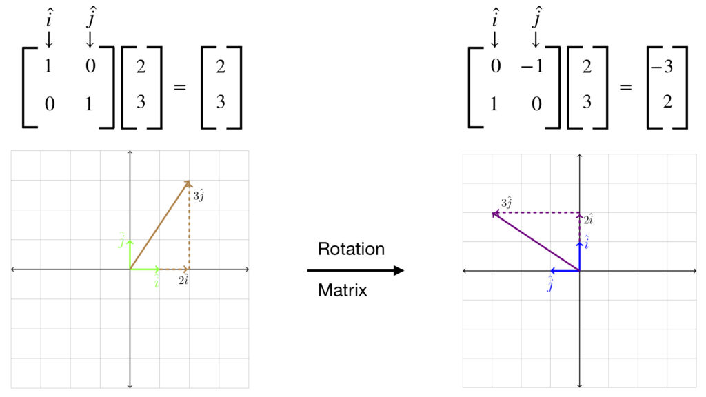
As in our previous discussion about linear transformations, the essence of what’s happening in this operation is that the rotation matrix, $A$ , changes the basis vectors from those of the Cartesian coordinate system specified by the identity matrix to a coordinate system specified by matrix $A$ : $\hat{i}=\begin{bmatrix}1\\0\end{bmatrix}$ to $\hat{i}=\begin{bmatrix}-1\\\,\,\,\,\,0\end{bmatrix}$ and $\hat{i}=\begin{bmatrix}1\\0\end{bmatrix}$ to $\hat{i}=\begin{bmatrix}-1\\\,\,\,\,\,0\end{bmatrix}$ . Note that the left-hand columns of each matrix specify the basis vector $\hat{i}$ and the right-hand columns specify $\hat{j}$ . The vector upon which the identity matrix, $I$ , and $A$ “operate” is $\begin{bmatrix}2\\3\end{bmatrix}$ . When $I$ operates on this vector, it returns the same result. However, when $A$ acts on it, the result is $\begin{bmatrix}-3\\\,\,\,\,\,2\end{bmatrix}$ . This problem can be looked at from two viewpoints: the row viewpoint and the column viewpoint. The column viewpoint is illustrated in the diagram:

$2\hat{i} + 3\hat{j} = 2\begin{bmatrix}0\\1\end{bmatrix}+ 3\begin{bmatrix}-1\\\,\,\,\,\,0\end{bmatrix}= \begin{bmatrix}-3\\\,\,\,\,\,2\end{bmatrix}$

The second matrix considered in the video, which we’ll call $B$ , works by “stretching” vectors (i.e., it creates a so-called shear):

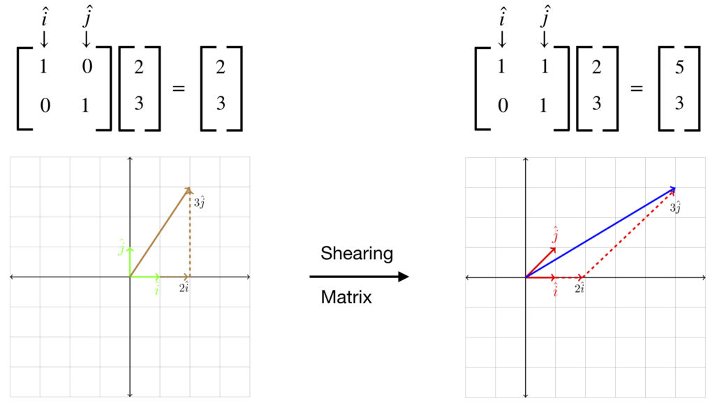
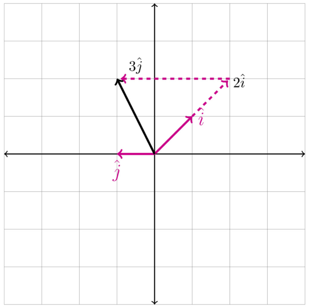
Again, the column viewpoint is illustrated in the diagram:

$2\hat{i} + 3\hat{j} = 2\begin{bmatrix}1\\0\end{bmatrix}+ 3\begin{bmatrix}1\\1\end{bmatrix}= \begin{bmatrix}5\\3\end{bmatrix}$

But what is the effect of first applying the rotation matrix, $A$ , on the vector $\begin{bmatrix}2\\3\end{bmatrix}$ , then applying the shearing matrix, $B$ (i.e., $AB\vec x=\vec b$ where $b$ is some unknown vector result, and in our example, $\vec x = \begin{bmatrix}2\\3\end{bmatrix}$ )? There are two ways to look at this.

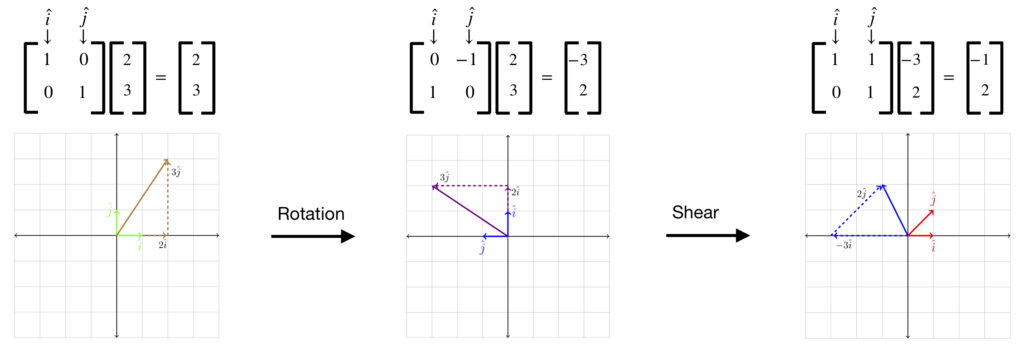
The first viewpoint is shown above. In the initial step of this method, the rotation matrix acts on $\begin{bmatrix}2\\3\end{bmatrix}$ to yield a new vector, $\begin{bmatrix}-3\\\,\,\,\,\,2\end{bmatrix}$ . The shearing matrix is then applied to $\begin{bmatrix}-3\\\,\,\,\,\,2\end{bmatrix}$ to give our final result, $\begin{bmatrix}-1\\\,\,\,\,\,2\end{bmatrix}$ . (We called $\begin{bmatrix}-1\\\,\,\,\,\,2\end{bmatrix}$ vector $\vec b$ in the equation $AB\begin{bmatrix}\vec x \end{bmatrix}=\vec b$ above).

The second viewpoint from which we can examine this problem is to multiply matrices $A$ and $B$ to make a new $C$ (which we’ll call a composite matrix) then allow this composite matrix to act on $\vec x$ to produce $\vec b$ . This process is worth examining in detail as this is the major point of this section.

Recall that each column of a matrix can be thought of as representing a basis vector. By multiplying 2 matrices together (say $A$ time $B$ , in that order), what’s actually happening is that $A$ is transforming (linearly) each basis vector specified in each column of $B$ into a new basis vector, and these new basis vectors are used to form the columns of a new matrix.

The first step in this process is shown below:

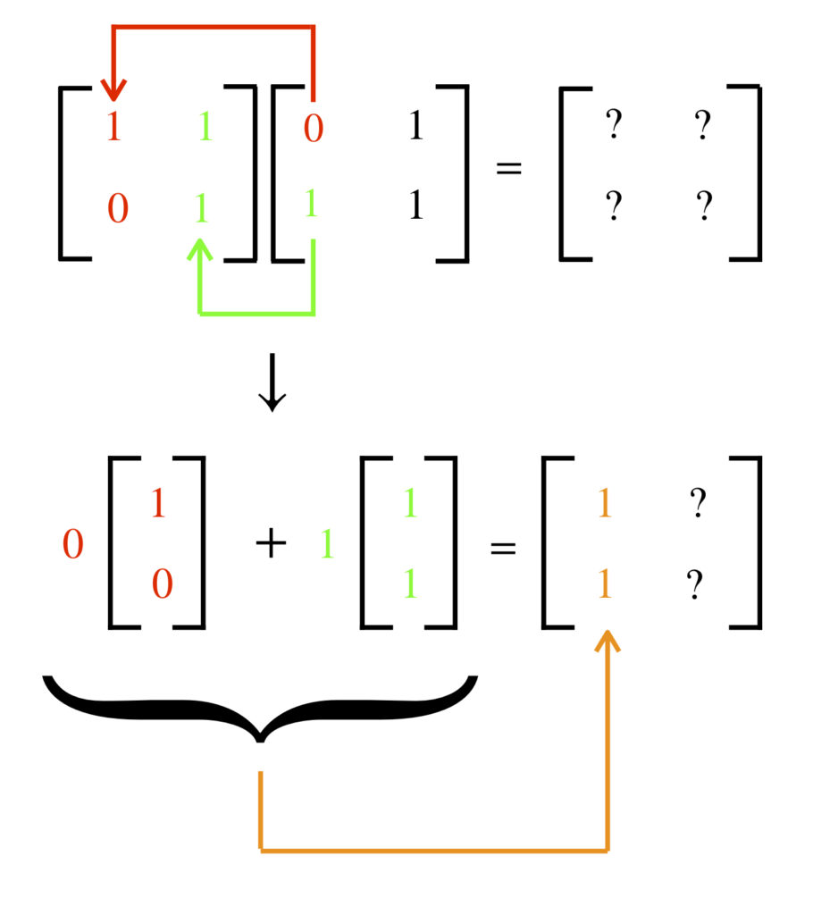
The second step occurs in a similar manner:

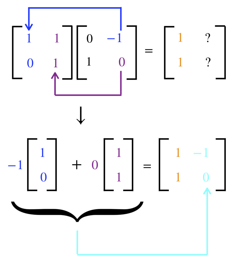
The end result is:

$\begin{bmatrix} 1&0\\1&1 \end{bmatrix}\begin{bmatrix} \,\,\,\,\,0&1\\-1&0 \end{bmatrix}= \begin{bmatrix} \,\,\,\,\,1&1\\-1&0 \end{bmatrix}$

Now multiply the composite matrix on the right, $C$ , with $\vec x = \begin{bmatrix} 2\\3 \end{bmatrix}$ . Just as when we sequentially applied $A$ on $\vec x={\begin{bmatrix} 2\\3 \end{bmatrix}$ , then applied $B$ on this result, we get $\begin{bmatrix} -1\\ \,\,\,2 \end{bmatrix}$ :

Algebraically, $C\vec x =\begin{bmatrix} \,\,\,\,\,1&1\\-1&0 \end{bmatrix} \begin{bmatrix} 2\\3 \end{bmatrix} = \begin{bmatrix} -1\\ \,\,\,2 \end{bmatrix}=\vec b$

The punchline of this discussion comes from comparing the result of multiplying matrices by the method resulting from the geometric argument described above with the rote mechanical multiplication algorithm described earlier. Here is the result obtained by the geometric argument:

This method can be thought of as the “column version” of matrix multiplication. In the first step (shown in the upper row), the $\hat{i}$ basis vector of $A$ is transformed by $B$ into a new basis vector which becomes the $\hat{i}$ basis vector of a new matrix. In the second step (shown in the lower row, the $\hat{j}$ basis vector of $A$ is transformed by $B$ into a new basis vector which becomes the $\hat{j}$ basis vector of the new matrix.

Compare this with the rote technique described in the section entitled Matrix times matrix.

This method can be thought of as the “row version” of matrix multiplication. In the first step, the dot product is taken between the left-hand column of $B$ and the top row of $A$ . The result becomes the $1,1$ entry of a new matrix. Next, the dot product is taken between the the left-hand column of $B$ and the bottom row of $A$ . The result becomes the $1,2$ entry of the new matrix. The process is then repeated by dotting the right-hand column of $B$ with the top and bottom rows of $A$ to yield the $2,1$ and $2,2$ entries of $C$ , respectively .

Note that the result from both the method derived from the geometric argument and the rote method produce the same result, matrix $C$ . Few would debate that the rote method is a faster/more efficient way to do matrix multiplication. However, it is worthwhile to see the geometric interpretation of matrix multiplication-at least once-to gain some intuition as to why the rote method works.

Commutation relationship between matrices

Let’s re-examine the 2-dimension example we’ve already been working with and see what happens if we change the order of matrix multiplication. Let $A$ be the rotation matrix $\begin{bmatrix}0&-1\\1&\,\,\,\,\,0\end{bmatrix}$ and $B$ the shearing matrix $\begin{bmatrix}1&0\\1&1\end{bmatrix}$ . The question we want to ask is, “Does $AB=BA$ ?” We already know that $AB=\begin{bmatrix}1&-1\\1&\,\,\,\,\,0\end{bmatrix}$ . We next need to calculate $BA$ . We’ll do it the easy way-by the rote method:

$BA=\begin{bmatrix}1&0\\1&1\end{bmatrix}\begin{bmatrix}0&-1\\1&\,\,\,\,\,0\end{bmatrix}=\begin{bmatrix}0&-1\\1&\,\,\,\,\,1\end{bmatrix}$

$\begin{bmatrix}1&-1\\1&\,\,\,\,\,0\end{bmatrix} \neq \begin{bmatrix}0&-1\\1&\,\,\,\,\,1\end{bmatrix}$ which means that $AB \neq BA$ . There’s a term for the quantity $AB-BA$ . It’s called the commutator of $A$ and $B$ . If the commutator, $AB-BA=0$ (i.e., $AB=BA$ ) it is said that matrices $A$ and $B$ commute. If $AB-BA \neq 0$ (i.e., $AB \neq BA$ ) as in the example we just examined, it is said that $A$ and $B$ do not commute.

Most of time, matrices do not commute, but at times, they do. For example, take the matrix $B=\begin{bmatrix}2&3\\1&4\end{bmatrix}$ . To find a matrix (or matrices), $A$ , that commute(s) with $B$ , we do the following:

Let $B=\begin{bmatrix}2&3\\1&4\end{bmatrix}$ . Let $A=\begin{bmatrix}a&b\\c&d\end{bmatrix}$ . If the two matrices commute, then

$\begin{bmatrix}a&b\\c&d\end{bmatrix}\begin{bmatrix}2&3\\1&4\end{bmatrix}=\begin{bmatrix}2&3\\1&4\end{bmatrix}\begin{bmatrix}a&b\\c&d\end{bmatrix}$

$\begin{bmatrix}a&b\\c&d\end{bmatrix}\begin{bmatrix}2&3\\1&4\end{bmatrix}=\begin{bmatrix}2a+b & 3a+4b\\2c+d & 3c+4b \end{bmatrix}$

And

$\begin{bmatrix}2&3\\1&4\end{bmatrix}\begin{bmatrix}a&b\\c&d\end{bmatrix}=\begin{bmatrix}2a+3c & 2b+3d\\a+4c & b+4d \end{bmatrix}$

Because $AB=BA$ , each entry of $AB$ should equal its corresponding entry from $BA$ . This gives us the following 4 equations in 4 unknowns:

$\begin{align*} 2a+b &= 2a+3c \Rightarrow b=3c \\ 3a+4b &= 2b+3d \Rightarrow 3a+2b=3d \Rightarrow 3a+2(3c)=3d \Rightarrow 3a+6c=3d \Rightarrow a+2c=d \\2c+d &= a+4c \Rightarrow d=a+2c \\3c+4d &=b+4d \Rightarrow 3c=b \end{align*}$

The top and bottom equations are the same. The second and third equations are also the same. Therefore, we’re left with the following 2 equations:

$\begin{align*} b &= 3c \\ a+2c&=d \end{align*}$

So, a matrix that will commute with $\begin{bmatrix}2&3\\1&4\end{bmatrix}$ takes this form:

$\begin{bmatrix}a&3c\\c&a+2c\end{bmatrix}$

That means that we can choose any numbers for values of $a$ and $c$ . As long as the above relationships are maintained, matrix $A$ will commute with matrix $B$ .

For example, let $a=7$ and $c=1$ . Then the matrix, $B=\begin{bmatrix}2&3\\1&4\end{bmatrix}$ should commute with the following matrix (we’ll call it $A$ ):

$\begin{bmatrix}7&3(1)\\1&7+2(1)\end{bmatrix}=\begin{bmatrix}7&3\\1&9\end{bmatrix}$

Let’s check it out:

$\begin{align*}AB&=\begin{bmatrix}7&3\\1&9\end{bmatrix}\begin{bmatrix}2&3\\1&4\end{bmatrix}\\&=\begin{bmatrix}7\cdot 2+3\cdot1 & 7\cdot3+3\cdot 4\\ 1\cdot 2+9\cdot1 & 1\cdot 3+9\cdot4 \end{bmatrix}\\&=\begin{bmatrix}14+3&21+12\\2+9&3+36\end{bmatrix}\\&=\begin{bmatrix}17&33\\11&39\end{bmatrix}\end{align*}$

and

$\begin{align*}BA&=\begin{bmatrix}2&3\\1&4\end{bmatrix}\begin{bmatrix}7&3\\1&9\end{bmatrix}\\&=\begin{bmatrix}2\cdot 7+3\cdot1 & 2\cdot3+3\cdot 9\\ 1\cdot 7+1\cdot4 & 1\cdot 3+4\cdot9 \end{bmatrix}\\&=\begin{bmatrix}14+3&6+27\\7+4&3+36\end{bmatrix}\\&=\begin{bmatrix}17&33\\11&39\end{bmatrix}\end{align*}$

So it works!

Solving matrix equations 1

The main method of solving matrix equations such as $A\vec x=\vec b$ or their equivalent, systems of linear equations, is Gaussian elimination. We’ve touched on this briefly when we’ve had to solve such systems. However, we will take a closer look at his method here.

The basic idea behind is to take an equation like this:

$\begin{bmatrix} \,m&\,m&\,m&\,m\\\,m&\,m&\,m&\,m\\\,m&\,m&\,m&\,m\\\,m&\,m&\,m&\,m\end{bmatrix}\begin{bmatrix} x_1\\x_2\\x_3\\x_4\end{bmatrix}= \begin{bmatrix} b_1\\b_2\\b_3\\b_4\end{bmatrix}$ and turn it into an equation like this:

$\begin{bmatrix} n_1&m&m&m\\0&n_2&m&m\\0&0&n_3&m\\0&0&0&n_4\end{bmatrix}\begin{bmatrix} x_1\\x_2\\x_3\\x_4\end{bmatrix} = \begin{bmatrix} c_1\\c_2\\c_3\\c_4\end{bmatrix}$

where the $m's$ are some number (that can include 0) and the $n's$ are numbers other than 0.

We’ll call the matrix with all $m's$ $A$ . We’ll call the matrix a combination of $n's$ , $m's$ and $0's$ $U$ because it is what’s called an upper triangular matrix. That means that 1) the upper right-hand portion of the matrix, which forms a triangle, consists of non-zero numbers along its diagonal and other numbers (zero or non-zero) above and to the right of the diagonal while 2) the lower left-hand portion of $U$ is all 0’s. The dot product of \vec x with the bottom row of $U$ gives $n_4$ (a number) time $x_4$ (a variable), and that is equal to another number, $c_4$ , the bottom entry in a new vector, $\vec c$ . This equation allows us to solve for $x_4$ . The value of $x_4$ is then back-substituted into the equation above it to solve for $x_3$ ; the values of $x_3$ and $x_4$ are substituted into the second from top equation to solve for $x_2$ ; and finally, the values of $x_2$ , $x_2$ and $x_4$ are back-substituted into the top equation to get the value of $x_1$ . That solves the system of equations.

This algorithm is illustrated by the following example:

$\begin{align*} 2x-3y&=3\\4x-5y+z&=7\\2x-y-3z&=5 \end{align*}$

Multiply the top equation by 2 and subtract it from equation 2. We get:

$\begin{align*} 2x-3y&=3\\y+2&=1\\2x-y-3z&=5 \end{align*}$

Subtract the top equation from the bottom equation. That gives:

$\begin{align*} 2x-3y&=3\\y+2&=1\\2y-3z&=2 \end{align*}$

Multiply the middle equation by 2 and subtract it from it from bottom equation. We’re left with:

$\begin{align*} 2x-3y&=3\\y+2&=1\\-5z&=0 \end{align*}$

So $z=0$ . Back-substitute $z=0$ into the middle equation:

$y+z=1 \Rightarrow y+0=1 \Rightarrow y=1$

Back-substitute $y=1$ into the top equation. That leaves:

$2x-3y=3 \Rightarrow 2x-3\cdot 1 =3 \Rightarrow 2x=6 \Rightarrow x=3$

The same system of equations represented in matrix equation form is:

$\begin{bmatrix} 2&-3&\,\,\,0\\4&-5&\,\,\,1\\2&-1&-3 \end{bmatrix}\begin{bmatrix} x\\y\\z \end{bmatrix}=\begin{bmatrix} 3\\7\\5 \end{bmatrix}$

What we’re manipulating when we do Gaussian elimination is numbers-specifically the coefficients of the variables, $x$ , $y$ and $z$ and the numbers on the right-hand side of the equal sign. Therefore, we can create a short-hand for doing Gaussian elimination that will make the process more efficient:

$\begin{array}{rrr|r}2 &-3&0&3\\4 &-5& 1&7\\2 &-1& -3&5 \end{array}\quad\rightarrow\quad \begin{array}{rrr|r}2 &-3&0&3\\0 &1& 1&1\\0 &2& -3&2 \end{array}\quad\rightarrow\quad\begin{array}{rrr|r}2 &-3&0&3\\0 &1& 1&1\\0 &0& -5&0 \end{array}$

The numbers to the left of the vertical line are matrix elements. The numbers to the right of the vertical line are “the answers” to the 3 equations, if you’re taking the row viewpoint, or the coefficients of the resultant vector, if you’re taking the column viewpoint. We could equally just place all of these numbers into one matrix, called an augmented matrix, and proceed as we did above, as long as we remember that the number to the far right is equivalent to the number to the right of the vertical line in our other shorthand (not too hard to do):

$\begin{bmatrix} 2 &-3&\,\,\,\,\,0&3\\4 &-5& \,\,\,\,\,1&7\\2 &-1& -3&5 \end{bmatrix}$

Here are a few key facts about the solutions we get from the process of Gaussian elimination:

If Gaussian elimination yields a matrix like that pictured above-an upper triangular matrix with numbers on the diagonal elements (called pivots)-then the system of equations will have one specific solution.
If Gaussian elimination winds up with a row that says 0 equals some number, then there will be no solution.
If Gaussian elimination ends up with a row that says 0 = 0, then the system of equations will have an infinite number of solutions.

The last two bullet points are probably worth some additional explanation. Remember, the matrix representation of a system of equations represents just that-equations. Say we have a system of equations with three variables. Say we wind up with a row of zeros in our last row. That means

$0x+0y+0z=0$

We could put in any number in for any of the variables. Therefore, there are an infinite number of solutions.

Likewise, if we have something like this:

$0x+0y+0z=5$

No matter what numbers we put in for any of the variables, that equation will never be true. Therefore, there is no solution to this system of equations.

All of the matrices we have considered so far are square matrices (i.e., # of rows = # of columns). Note that if such a matrix has just one solution, it’s called nonsingular. If it has no solution or an infinite number of solutions, it’s called singular. Note also that the first nonzero entry in a given row is called a pivot. From the above discussion, it is evident that if, after elimination, there are non-zero numbers in every diagonal position (i.e, all of the diagonal entries are pivots), then the matrix will be nonsingular. If there is a row of zeros in the matrix, then there necessarily will be a 0 on a diagonal entry. In such a case, then, that matrix has to be singular (since we’ll wind up with a row that gives us 0 = 0 or 0 = some nonzero number, which mean an infinite number of solutions or zero solutions, respectively). We’ll have more to say about nonsingular and singular matrices later.

The above example makes use of multiplying and subtracting equations to perform elimination. We could also add equations. Strang’s textbook follows the convention of subtracting equations rather than adding, noting that multiplying by -1 then subtracting has the same effect as adding. In some cases, adding equations may be preferable, especially when using augmented matrices (discussed below) to solve equations. For continuity, we’ll generally subtract one equation from another, noting when we use addition instead.

The other technique that can sometimes be useful is to exchange rows. The following example, taken from Strang’s textbook, illustrates this latter technique:

$\begin{align*} x+2y+2z&=1\\4x+8y+9z&=3\\3y+z&=1 \end{align*}$

In augmented matrix form, this becomes:

$\begin{bmatrix} 1&2&2&1\\4&8&9&3\\0&3&1&1 \end{bmatrix}$

Multiply the top equation by 4 and subtract it from the second equation to get a new second equation. That gives us:

$\begin{bmatrix} 1&2&2&\,\,\,\,\,1\\0&0&1&-1\\0&3&2&\,\,\,\,\,1 \end{bmatrix}$

At this point, rather than performing multiplication/subtraction step between the top and bottom equations then another multiplication/subtraction step between the middle and bottom rows, it’s easier to just exchange the middle and bottom rows. That yields:

$\begin{bmatrix} 1&2&2&\,\,\,\,\,1\\0&3&2&\,\,\,\,\,1\\ 0&0&1&-1\end{bmatrix}$

Now take the coefficients and numbers specified by the matrix above and convert them back into equations:

$\begin{align*} x+2y+2z&=\,\,\,\,\,1\\3y+2z&=\,\,\,\,\,1\\z&=-1 \end{align*}$

$\begin{align*} \mathbf{z}\mathbf{&=}\mathbf{-1}\\3y+2(-1)&=\,\,\,1 \Rightarrow3y-2=1\Rightarrow 3y=3\Rightarrow \mathbf{y=1}\\x+2(1)+2(-1)&=\,\,\,1\Rightarrow x+0=1\Rightarrow \mathbf{x=1} \end{align*}$

We can also create matrices that bring about row multiplication/subtraction steps and row exchanges. The basic idea is to modify the identity matrix to produce these results. Recall that the identity matrix, $I$ when multiplied by any other matrix, returns the original matrix. Therefore, we have but to change one other entry in $I$ to produce a multiplication/subtraction step or row exchange.

Following the lead of Strang’s text, we’ll call a matrix that produces a multiplication/subtraction (or addition) step an elimination matrix, $E$ , and a matrix that produces a row exchange a permutation matrix, $P$ . Suppose we want to apply a multiplication/subtraction step (let’s call such a step an elimination step) by applying $E$ on some matrix (call it $A$ ). We want to eliminate a term from an equation represented by some row in $A$ (call it row b) by subtracting the analogous term from another row in $A$ , (call it row a). To do this, we multiply the coefficient for the term in row a by a multiplication factor, $m$ , such that, when we subtract row a from row b, the coefficient for the term in question becomes zero.

Because of the mechanics of matrix multiplication,

the column of $I$ that is modified to make $E$ determines which row in $A$ is multiplied, and
the row of $I$ that is modified to make $E$ determines which row in $A$ the recently multiplied row is subtracted from

Hopefully, applying this algorithm to the augmented matrix example we’ve recently considered will make the meaning of this jumble of words more clear.

In that example, we want to multiply the first row of $A$ by 4 and subtract it from the second row of $A$ . To do this,

we modify the column 1 of $I$ (because row 1 of $A$ is the row we want to multiply); then
we modify row 2 of column 1 of $I$ because row 2 of $A$ is the row we want to subtract row 1 from
That is, we modify the $I_{i,j}=I_{1,2}$ entry of $I$

How do we modify this entry? By replacing the existing 0 at $I_{1,2}$ with our multiplier, $m$ . And what is $m$ in this case? Well, we want to multiply row 1 by 4 so the magnitude of $m$ is 4; and we want to subtract row 1 from row 2 so we make $m$ negative (i.e., $m=-4$ ).

In matrix format, here’s the transformation we made in $I$ to get $E$ (which we’ll call $E_{1,2}$ to reflect the column and row we manipulated):

$\begin{bmatrix}1&0&0\\0&1&0\\0&0&1\end{bmatrix} \rightarrow \begin{bmatrix}\,\,\,\,\,1&0&0\\-4&1&0\\\,\,\,\,\,0&0&1\end{bmatrix}$

Now multiply $E_{1,2}A$ . The mechanics of doing this should give a clearer picture of why the elimination matrix does what it does:

$\begin{bmatrix}\,\,\,\,\,1&0&0\\-4&1&0\\\,\,\,\,\,0&0&1\end{bmatrix}\begin{bmatrix} 1&2&2&1\\4&8&9&3\\0&3&1&1 \end{bmatrix}=\begin{bmatrix} 1&2&1&\,\,\,\,\,1\\0&0&1&-1\\0&3&2&\,\,\,\,\,1 \end{bmatrix}$

As alluded to above, we can also make a matrix, $P$ (called a permutation matrix) that will operate on a matrix to bring about a row exchange in that matrix. Again, this is done by modifying the identity matrix, $I$ . Specifically, because, just as with elimination matrices, columns affect rows and rows affect columns, to swap 2 rows, we look for columns with the same numbers as the rows that we want to swap, then switch the position of the 1’s in those columns, keeping those 1’s in the same row.

To illustrate this, we’ll stick with the example on which we’ve been working. In this example, we want to exchange rows 2 and 3. To create a matrix that makes this change, we find the columns of the same number as the rows we want to exchange-that would be columns 2 and 3. The 1 in column 2 is in row 2. To facilitate the row exchange, we move that 1 from the second to third column of row 2. This is because, when each column of $A$ is dotted with the second row of $P$ , the only term that will produce anything other that 0 is the third term, the term that contains a 1 times a contribution from the third row of $A$ . When this occurs, the entry from the third row of $A$ becomes the corresponding column of row 2 in a new matrix that is the product of $P$ and $A$ .

Likewise, the 1 in column 3 is in row 3. To finish making our permutation matrix, we take that 1 and move it from the third to the second column of row 3. By doing this, when we dot each column of $A$ with the third row of $P$ , the only term that produces any output to the new matrix is the second term. That’s because the second column of $P$ contains the 1; the other columns of the third row of $P$ contain 0’s and output nothing to the new matrix. And because that 1 is in the second column, it “selectively outputs” the values of row 2 of $A$ to row 3 of the new matrix.

As in the case of application of the elimination matrix, the above words are just gibberish until we actually see the matrices and perform the manipulations for ourselves:

$\begin{bmatrix} 1&0&0\\0&0&1\\0&1&0 \end{bmatrix}\begin{bmatrix} 1&2&2&\,\,\,\,\,1\\0&0&1&-1\\0&3&2&\,\,\,\,\,1 \end{bmatrix}=\begin{bmatrix} 1&2&2&\,\,\,\,\,1\\0&3&2&\,\,\,\,\,1\\0&0&1&-1 \end{bmatrix}$

The total solution to this problem we’ve been working on with elimination and permutation matrices can be written as follows:

$P_{k,l}E_{i,j}A=P_{k,l}E_{i,j}\vec b;\quad \rightarrow \quad P_{2,3}E_{2,1}A=P_{2,3}E_{2,1}\vec b$

The convention used in Strang’s text is that $i$ is the row we’re multiplying and $j$ is the equation we’re subtracting $i$ from. The order of the subscripts associated with the permutation matrix, $k$ and $l$ , doesn’t matter.

Recall that the order of multiplication of the matrices in this expression does matter. The multiplication steps need to be carried out right to left.

Recall, also, that $P_{k,l}$ and $E_{i,j}$ can be multiplied together to form a new matrix-let’s call it $E$ without subscripts. Then,

$E=P_{k,l}E_{i,j}\quad \rightarrow \quad E=P_{2,3}E_{2,1}$ :

$E=\begin{bmatrix}1&0&0\\0&0&1\\0&1&0\end{bmatrix}\begin{bmatrix}\,\,\,\,\,1&0&0\\-4&1&0\\\,\,\,\,\,0&0&1\end{bmatrix}=\begin{bmatrix}\,\,\,\,\,1&0&0\\\,\,\,\,\,0&0&1\\-4&1&0\end{bmatrix}$

And

$EA=E\vec b$

Non-square matrices

So far, all of the matrices we’ve been working with have been square matrices-that is, matrices with the same number of rows and columns. Obviously, there are many occasions where there are either more rows than columns or more columns than rows. We can still do elimination. Instead of there being pivots on diagonal elements, the matrix looks more like a staircase but still with numbers in the right upper aspect and zeros in the lower left portion. We called the upper triangular matrix we obtained after elimination (and from which we solved our system of equation, if a solution existed) U. We call the matrix we obtain after elimination with a rectangular matrix an echelon form of $U$ . We still call the nonzero entries of each row pivots. If we reduce the matrix further such that the pivots of the echelon matrix equal 1, then we call such a matrix the reduced row echelon matrix form (rref or R). Here is an example:

$A=\begin{bmatrix}1&2&2&4\\3&8&6&16\end{bmatrix}$

Subtract 3 times row 1 from row 2:

echelon form of $U=\begin{bmatrix}1&2&2&4\\0&2&0&4\end{bmatrix}$

Subtract row 2 of $U$ from row 1 of $U$ then divide row 2 of $U$ by 2. We get:

$R=rref=\begin{bmatrix}1&0&2&0\\0&1&0&2\end{bmatrix}$

Special solutions

Here’s another example. Consider the following matrix:

$A=\begin{bmatrix}1&1&2&3\\2&2&8&10\\3&3&10&13\end{bmatrix}$

We want to find the null space (see below) of this matrix (that is, all of the solutions for $\vec x$ that solve the following equation: $A\vec x = 0$ ).

We perform elimination. First, subtract 2 times row 1 from row 2 and 3 times row 1 from row 3. That gives us

$A^\prime=\begin{bmatrix}1&1&2&3\\0&0&4&4\\0&0&4&4\end{bmatrix}$

Subtract row 2 from row 3. That leaves

$U=\begin{bmatrix}1&1&2&3\\0&0&4&4\\0&0&0&0\end{bmatrix}$

Divide row 2 by 4:

$U=\begin{bmatrix}1&1&2&3\\0&0&1&1\\0&0&0&0\end{bmatrix}$

We have a row of 0’s so we know that there are an infinite number of solutions to this equation but let’s try to be a bit more specific. We note that we have two pivots (a nonzero number in a row with no other nonzero numbers to its left). We also have two columns that contain no pivots (columns 2 and 4). If the vector $\vec x$ that we’re multiplying $A$ by has components $x_1,\,x_2,\,x_3,\,x_4$ , then the components that multiply the non-pivot columns, $x_2$ and $x_4$ , are called free variables. To get the solution we want, called special solutions, we

take a non-pivot variable
assign that variable a value of 1 and assign a value of 0 to all of the other free variables
back-substitute those values into the nonzero rows of $U$ or $R$ ; that yields one special solution
to find the others, repeat the above process with each of the other free variables

In our case,

$x_1+x_2+2x_3+3x_4=0$

Choose $x_2=1$ and $x_4=0$ . We get

$\begin{array}{rcl}x_3+3\cdot 0&=&0 \quad \Rightarrow \quad x_3=0\\ x_1+1+2\cdot 0+3\cdot 0&=&0 \quad \Rightarrow \quad x_1=-1\end{array}$

So the first special solution is $x_2 \begin{bmatrix} -1\\\,\,\,\,\,1\\\,\,\,\,\,0\\\,\,\,\,\,0 \end{bmatrix}$

Next, choose $x_2=0$ and $x_4=1$ . That gives us

$\begin{array}{rcl}x_3+1\cdot 1&=&0 \quad \Rightarrow \quad x_3=-1\\ x_1+0+2\cdot -1+3\cdot 1&=&0 \quad \Rightarrow \quad x_1=-1\end{array}$

So the second special solution is $x_4 \begin{bmatrix} -1\\\,\,\,\,\,0\\-1\\\,\,\,\,\,1 \end{bmatrix}$

The complete special solution, then, is

$x=x_2 \begin{bmatrix} -1\\\,\,\,\,\,1\\\,\,\,\,\,0\\\,\,\,\,\,0 \end{bmatrix}+x_4 \begin{bmatrix} -1\\\,\,\,\,\,0\\-1\\\,\,\,\,\,1 \end{bmatrix}=\begin{bmatrix} -x_2-x_4\\x_2\\-x_4\\x_4 \end{bmatrix}$

Inverse matrix

The relationship between matrix type (i.e., singular vs. nonsingular) and the inverse matrix merits some discussion. But before we can actually discuss this, we need to lay some groundwork.

Definitions:

Definition 1: If $AB=I$ and $BA=I$ then $B$ is called the inverse of $A$ and the matrix $A$ is referred to as being invertible. The symbol for the inverse of $A^-1$ . So $AA^-1=I$ and $A^-1A=I$ . Here’s an example:

$\begin{array}{rcl}\begin{bmatrix} \,\,\,\,\,1&0&0\\-5&1&0\\\,\,\,\,\,0&0&1 \end{bmatrix}\begin{bmatrix} 1&0&0\\5&1&0\\0&0&1 \end{bmatrix}&=&\begin{bmatrix}\,\,\,\,\, 1\cdot 1 + 0\cdot 5+0\cdot 0&\,\,\,\,\,1\cdot 0+0\cdot 1+0\cdot 0&\,\,\,\,\,1\cdot 0+0\cdot 0+0\cdot 1\\-5\cdot 1+1\cdot 5+0\cdot 0&-5\cdot 0+1\cdot 1+0\cdot 0&-5\cdot 0+1\cdot 0+0\cdot 1\\\,\,\,\,\,0\cdot 1+0\cdot 1+1\cdot 0&\,\,\,\,\,0\cdot 0+0\cdot 1+0\cdot 0&\,\,\,\,\,0\cdot 0+0\cdot 0+1\cdot 1 \end{bmatrix}\\&=&\begin{bmatrix} 1&0&0\\0&1&0\\0&0&1 \end{bmatrix}\end{array}$

Definition 2: A square matrix (i.e., # of rows = # of columns) $A$ is nonsingular iff (if and only if) the only solution to $A\vec x=0$ is $\vec x = 0$ . Otherwise, $A$ is singular.

Proofs:

If $A$ and $B$ are square matrices that are nonsingular, then $AB$ is also nonsingular.

(taken from https://yutsumura.com/two-matrices-are-nonsingular-if-and-only-if-the-product-is-nonsingular/#more-4875)

If $AB$ is nonsingular, then $B$ is nonsingular.

(taken from https://yutsumura.com/two-matrices-are-nonsingular-if-and-only-if-the-product-is-nonsingular/#more-4875)

If $A$ is nonsingular, then the columns of $A$ are linearly independent.

(taken from https://yutsumura.com/two-matrices-are-nonsingular-if-and-only-if-the-product-is-nonsingular/#more-4875)

$A$ is nonsingular iff $A\vec x = \vec b$ has a unique solution for $\vec b \in \mathbb{R}^4$ .

(taken from https://yutsumura.com/two-matrices-are-nonsingular-if-and-only-if-the-product-is-nonsingular/#more-4875)

If $A$ is nonsingular, then $A$ is invertible

(taken from https://yutsumura.com/a-matrix-is-invertible-if-and-only-if-it-is-nonsingular)

If $A$ is invertible, then $A$ is nonsingular

(taken from https://yutsumura.com/a-matrix-is-invertible-if-and-only-if-it-is-nonsingular)

If $AB$ is nonsingular, then $A$ is also nonsingular.

(taken from https://yutsumura.com/two-matrices-are-nonsingular-if-and-only-if-the-product-is-nonsingular/#more-4875)

If $B$ is singular, then $AB$ is singular

(taken from href=”https://users.math.msu.edu/users/hhu/309/3091418.pdf

If $A$ is singular, then $AB$ is singular

If $AB$ is singular, then either $A$ , $B$ or both are singular

Calculating A^-1: Gauss-Jordan elimination

Technique

The inverse of a matrix can be calculated in various ways. A common method is Gauss-Jordan elimination. The basic idea is this: for some $n\,\text{x}\,n$ matrix, $A$ ,

We want to find a matrix, $A^{-1}$ , such that $AA^{-1}=I$
This is tantamount to solving the following equation
- $A\underbrace{\begin{bmatrix}x_1&\cdots&x_i&\cdots&x_n\\ \vdots&\,&\vdots&\,&\vdots \\ \vdots&\,&\vdots&\,&\vdots \\ \vdots&\,&\vdots&\,&\vdots \\n&\dots&n&\dots&n\end{bmatrix}}_{A^{-1}}=\underbrace{\begin{bmatrix}1&\dots&0&\dots&0\\ \vdots&\,&\vdots&\,&\vdots \\ 0&\,&1&\,&0 \\ \vdots&\,&\vdots&\,&\vdots \\0&\cdots&0&\cdots&1\end{bmatrix}}_{I}$
To solve this equation, we need to multiply each column of $A^{-1}$ , (which we’ll call $\mathbf{x_i}$ ) with $A$ to get the corresponding column of $I$ (which we’ll call $\mathbf{e_i}$ ). Thus, we need to solve $A\mathbf{x_1}=\mathbf{e_1}\text{, } A\mathbf{x_2}=\mathbf{e_2}\text{, } \dots \, A\mathbf{x_n}=\mathbf{e_n}$ .
How do we do this? By elimination.
We set up an augmented matrix with $A$ on the left and $I$ on the right, then proceed with elimination, as usual, until we have an upper triangular matrix on the left and a modification of the identity matrix on the right-a thing that looks something like this:
$\left[\begin{array}{ccc|ccc}x&x&x&1&0&0\\0&x&x&y&1&0\\0&0&x&y&y&1\end{array}\right]$
We then continue with elimination, adding/subtracting lower rows from upper rows from on the left side, until we get something that looks like this:
$\left[\begin{array}{ccc|ccc}x&0&0&u&u&u\\0&x&0&u&u&u\\0&0&x&u&u&u\end{array}\right]$
We then divide each row by $x$ . We are left with something like this:
$\left[\begin{array}{ccc|ccc}1&0&0&v&v&v\\0&1&0&v&v&v\\0&0&1&v&v&v\end{array}\right]$
Recall that each elimination step can be represented by a matrix, $E_i$ . So what we’ve really done here is multiplied the augmented matrix we started with by $E_1$ , $E_2$ , $\dots$ $E_n$ .
But also remember that multiplying by several elimination matrices is equivalent to multiplying by a single combined matrix that is the product of those elimination matrices. In this case, that combined matrix is $A^{-1}$ .
So we started with $\left[\begin{array}{c|c}A&I\end{array}\right]$ and ended with $\left[\begin{array}{c|c}I&A^{-1}\end{array}\right]$
How did we do this? We multiplied by $E_1$ , $E_2$ , $\dots$ $E_n$ = $A^{-1}$ :
$A^{-1}\left[\begin{array}{c|c}A&I\end{array}\right]=\left[\begin{array}{c|c}I&A^{-1}\end{array}\right]$

Example

Here is an example (taken from Strang, p. 84) to illustrate the technique:

$\begin{array}{rcl}\left[A\,\,\mathbf{e_1}\,\,\mathbf{e_2}\,\,\mathbf{e_3}\right]&=&\begin{bmatrix} \,\,\,\,\,2&-1&\,\,\,\,\,0&1&0&0\\-1&\,\,\,\,\,2&-1&0&1&0\\ \,\,\,\,\,0&-1&\,\,\,\,\,2&0&0&1 \end{bmatrix}\textbf{ Start Gauss-Jordan on A}\\ \,&\,&\, \\ &\rightarrow &\begin{bmatrix} \,\,\,\,\,2&-1&\,\,\,\,\,0&1&0&0 \\ \,\,\,\,\,\mathbf{0}&\,\,\,\,\,\mathbf{\frac32}&\mathbf{-1}&\mathbf{\frac12}&\mathbf{1}&\mathbf{0}\\ \,\,\,\,\,0&-1&\,\,\,\,\,2&0&0&1 \end{bmatrix}\,\, \frac12\textbf{ row 1}+\textbf{ row 2} \\ \,&\,&\, \\ U &=& \begin{bmatrix} \,\,\,\,\,2&-1&\,\,\,\,\,0&1&0&0 \\ \,\,\,\,\,0& \,\,\,\,\,\frac32&-1&\frac12&1&0\\ \,\,\,\,\,\mathbf{0}&\,\,\,\,\,\mathbf{0}&\,\,\,\,\,\mathbf{\frac43}&\mathbf{\frac13}&\mathbf{\frac23}&\mathbf{1} \end{bmatrix}\,\, \frac23}\textbf{ row 2}+\textbf{ row 3} \\ &\rightarrow& \begin{bmatrix} \,\,\,\,\,2&-1&\,\,\,\,\,0&1&0&0 \\ \,\,\,\,\, \mathbf{0}& \,\,\,\,\,\mathbf{\frac32}&\,\,\,\,\,\mathbf{0}&\mathbf{\frac34}&\mathbf{\frac32}&\mathbf{\frac34}\\ \,\,\,\,\,0&\,\,\,\,\,0&\,\,\,\,\,\frac43&\frac13&\frac23&1 \end{bmatrix}\,\, \frac34}\textbf{ row 3}+\textbf{ row 2} \\ \,&\,&\, \\ &\rightarrow& \begin{bmatrix} \,\,\,\,\,\mathbf{2}&\,\,\,\,\,\mathbf{0}&\,\,\,\,\,\mathbf{0}&\mathbf{\frac32}&\mathbf{1}&\mathbf{\frac12} \\ \,\,\,\,\, 0& \,\,\,\,\,\frac32&\,\,\,\,\,0&\frac34&\frac32&\frac34\\ \,\,\,\,\,0&\,\,\,\,\,0&\,\,\,\,\,\frac43&\frac13&\frac23&1 \end{bmatrix} \,\,\, \begin{matrix} \textbf{divide by }2 \, \\ \textbf{divide by }\frac32 \\ \textbf{divide by }\frac43 \\ \end{matrix} \\ \,&\,&\, \\ &\rightarrow& \begin{bmatrix} \,\,\,\,\,\mathbf{1}&\,\,\,\,\,0&\,\,\,\,\,0&\mathbf{\frac34}&\mathbf{\frac12}&\mathbf{\frac14} \\ \,\,\,\,\, 0& \,\,\,\,\,\mathbf{1}&\,\,\,\,\,0&\mathbf{\frac12}&\mathbf{1}&\mathbf{\frac12}\\ \,\,\,\,\,0&\,\,\,\,\,0&\,\,\,\,\,\mathbf{1}&\mathbf{\frac14}&\mathbf{\frac12}&\mathbf{\frac34} \end{bmatrix} \,\,\,\begin{matrix} \text{=}&\left[I\,\,\mathbf{x_1}\,\,\mathbf{\,x_2}\,\,\mathbf{x_3}\right]&\text{=}\,\,\left[I\,\,A^{-1}\right] \end{matrix} \end{array}$

$\begin{bmatrix} \mathbf{\frac34}&\mathbf{\frac12}&\mathbf{\frac14} \\ \mathbf{\frac12}&\mathbf{1}&\mathbf{\frac12}\\ \mathbf{\frac14}&\mathbf{\frac12}&\mathbf{\frac34} \end{bmatrix}=A^{-1}$

Just a quick glimpse at a topic that will by considered in depth shortly: note that,

The product of the pivots of $A$ , $2(\frac32)(\frac43)=4$ . This product, $4$ , is called the determinant of $A$ .
involves division by the determinant
- $A^{-1}= \frac1{\text{det}} \begin{bmatrix} 3&2&1 \\ 2&4&2 \\ 1&2&3 \end{bmatrix} =\frac14 \begin{bmatrix} 3&2&1 \\ 2&4&2 \\ 1&2&3 \end{bmatrix}$

One final comment regarding Gauss-Jordan elimination that may seem obvious, but just a reminder: Gauss-Jordan elimination can only be applied to a matrix to find its inverse if the matrix

is nonsingular (since nonsingular matrices are the only type of matrix that have an inverse) and
is a square matrix (since the only type of matrix that can be nonsingular is a square matrix)

Now that we have discussed singular, nonsingular and inverse matrices, a few miscellaneous topics regarding the solutions to matrix equations need to be discussed.

PA = LU

A significant issue in linear algebra is attempting to solve the equation $A\mathbf{x}=\mathbf{b}$ . To do this, we apply Gaussian elimination. In Gaussian elimination, each step can be affected by multiplying a matrix, $E_i$ , on the left, times $A$ and $\mathbf{b}$ . So we have,

$\underbrace{E_n\,\dots\,E_2\,E_1\,A}_{U}\underbrace{\mathbf{x}}_{\mathbf{x}}=\underbrace{E_n\,\dots\,E_2\,E_1\,\mathbf{b}}_{\mathbf{c}}$

Note that in the above equation, as discussed in the section on the commutation relationship between matrices, the order in which we multiply the $E_i$ ‘s matters. Based on what we learned in the section on inverse matrices, we know that we can get $A$ back by multiplying both sides of the equation by the inverse of $U$ , which we’ll call $L$ (because it turns out that $L$ is always lower triangular):

$\underbrace{E^{-1}_n\,\dots\,E^{-1}_2\,E^{-1}_1}_{L}\,\underbrace{E_n\,\dots\,E_2\,E_1\,A}_{U}\underbrace{\mathbf{x}}_{\mathbf{x}}=\underbrace{E^{-1}_n\,\dots\,E^{-1}_2\,E^{-1}_1}_{L}\underbrace{E_n\,\dots\,E_2\,E_1\,\mathbf{b}}_{\mathbf{c}}$

Let’s let $E_{\text{tot}}$ be the product of the elimination matrices. From the above equation, we can see that,

$L\,E_{\text{tot}}\,A=IA=A$ and $E_{\text{tot}}\,A=U$ so $LU=A$ .

Let’s look at a couple of examples:

Consider the matrix $A=\begin{bmatrix}2&1\\6&8\end{bmatrix}$ . We perform elimination on this matrix by subtracting 3 times row 1 from row 2. The matrix that does this is $E_{21}\begin{bmatrix}\,\,\,\,\,1&0\\-3&1\end{bmatrix}$ . We have

$E_{21}\begin{bmatrix}\,\,\,\,\,1&0\\-3&1\end{bmatrix}\begin{bmatrix}2&1\\6&8\end{bmatrix}=\begin{bmatrix}2&1\\0&5\end{bmatrix}=U$

To get back from $A$ to $U$ , we multiply $U$ by the inverse of $E_{21}$ , $E^{-1}_{21}$ :

$E^{-1}_{21}E_{21}=\begin{bmatrix}1&0\\3&1\end{bmatrix}\begin{bmatrix}\,\,\,\,\,1&0\\-3&1\end{bmatrix}=\begin{bmatrix}1&0\\0&1\end{bmatrix}$

$E^{-1}_{21}E_{21}A=\begin{bmatrix}1&0\\3&1\end{bmatrix}\begin{bmatrix}\,\,\,\,\,1&0\\-3&1\end{bmatrix}\begin{bmatrix}2&1\\6&8\end{bmatrix}=\begin{bmatrix}1&0\\0&1\end{bmatrix}=AI=A\text{ and}$

$E^{-1}_{21}U=LU=\begin{bmatrix}1&0\\3&1\end{bmatrix}\begin{bmatrix}2&1\\0&5\end{bmatrix}=\begin{bmatrix}2&1\\6&8\end{bmatrix}=A$

Notice that the inverse of our elimination matrix, $E^{-1}$ (or $L$ ) is just our elimination matrix, $E$

Another way of looking at it is $U\mathbf{x}=\mathbf{c}$ and $L\mathbf{c}=\mathbf{b}$ .

Substitute $U\mathbf{x}$ for $\mathbf{c}$ in $L\mathbf{c}=\mathbf{b}$ . That leaves $LU\mathbf{x}}=\mathbf{b}$ .

But we also know that $A\mathbf{x}=\mathbf{b}$ . That means that $A\mathbf{x}=LU\mathbf{x}}$ which means that $A=LU$ .

Another form of $A=LU$ that some authors use is $A=LDU$ . (As will become evident below, the equation should more correctly be written $A=LDU^\prime$ but $A=LDU$ is the way most authors refer to it so we’ll stick with that.) In this form, we split $U$ into two matrices, one a diagonal matrix, $D$ that has the pivots of $U$ on its diagonals and a variant of $U$ (let’s call it $U^\prime$ ) that has all 1’s on its diagonals. When we multiply $DU^\prime$ we get back $U$ :

$U=\begin{bmatrix} d_1&\,&\,&\, \\ \,&d_2&\,&\, \\ \,&\,&\ddots&\, \\ \,&\,&\,& d_4 \end{bmatrix}\begin{bmatrix} 1&\frac{u_{12}}{d_1}&\frac{u_{13}}{d_1}&\cdot \\ \,&1&\frac{u_{23}}{d_2}&\cdot \\ \,&\,&\ddots&\vdots \\ \,&\,&\,& 1 \end{bmatrix}$

Extending the example we’ve already seen:

$LU=\begin{bmatrix}1&0\\3&1\end{bmatrix}\begin{bmatrix}2&1\\0&5\end{bmatrix}\text{ can be split into }LDU^\prime=\begin{bmatrix}1&0\\3&1\end{bmatrix}\begin{bmatrix}2&\,\\ \,&5\end{bmatrix}\begin{bmatrix}1&4\\0&1\end{bmatrix}$

$A=LU$ represents elimination without row exchanges. If we do our row exchanges before elimination, then $PA=LU$ where $P$ represents the product of all of the permutation matrices used to carry out the row exchanges. As we’ll see, this equation, $PA=LU$ , will become useful shortly.

Solving matrix equations 2

There are a few things that can be gleaned by examining $U$ , $R$ or $rref$ .

First, by way of review,

$U$ (short for upper triangular) is the matrix we get after application of Gaussian elimination to a square ( $n$ by $n$ ) matrix.
An echelon matrix is what we get after Gaussian elimination is performed on a rectangular matrix (i.e., an $m$ by $n$ matrix where $m\neq n$ ).
R is the row reduced echelon form ( $rref$ ) of a matrix after we’ve performed eliminations steps until all of the pivots are 1’s.
The pivots are the first non-zero entries on each row of $U$ , the echelon form of $U$ or $rref$ .

Then for a matrix, $A$ , that is reduced to $U$ , $R$ or $rref$ :

If there are nonzero entries on all of the diagonals of $U$ (i.e., all of the diagonal elements are pivots), then the matrix $A$ from which $U$ came is nonsingular. There will be a unique solution to $A\vec{x}=\vec{b}$ .
If there are any zeros along the diagonal of $U$ , then $A$ is singular. There will be none or many solutions to $A\vec{x}=\vec{b}$ .
If there is one or more rows of zeros in $U$ , then $A$ is singular.
If there is a row or column of zeros in $U$ , then the entries of the analogous row or column in $A$ are linearly dependent; on the other hand, if a row of $U$ has a pivot, then its entries are linearly independent.

Transpose of a matrix, A^T

The transpose of matrix $A$ is depicted by the mathematical symbol $A^T$ and is the result of swapping the rows and columns of $A$ . For example:

$A=\begin{bmatrix} a & b & c \\ d & e & f \\ g & h & i \end{bmatrix}\text{;} \quad A^T=\begin{bmatrix} a & d & g \\ b & e & h \\ c & f & i \end{bmatrix}$

An important theorem related to the transpose of matrices is its product rule:

$\mathbf{(AB)^T=B^TA^T}$

Here are two example designed to further show that this theorem works:

Vector Subspaces

Subspaces of a vector space, called vector subspaces, are an important topic that I don’t devote nearly enough time to in this article. However, here are some basic facts about them. For a given matrix, $A$ :

its column space is the set of all possible solutions (=vectors) that can be produced from all possible linear combinations of the columns of $A$ . It is represented symbolically as $C(A)$ .
its row space is the set of all possible solutions (=vectors) that can be produced from all possible linear combinations of the rows of $A$ . It is represented symbolically as $=C(A^T)$ where $A^T$ is the transpose of $A$ . The reason that this is true is because, by definition, when matrix $A$ is transposed, its rows become its columns. Thus, when we take all of the possible linear combinations of the columns of $A^T$ , what we’re really doing is taking all of the linear combinations of the rows of the original matrix, $A$ .
its nullspace is the set of all vectors, $\vec x$ , such that $A\vec x=0$ , 0 meaning the so-called zero vector, a vector with all 0’s for coefficients.
its left nullspace is the set of all vectors, $\vec x$ , such that $A^T\vec x=0$ , 0, again, representing the zero vector

There are two important properties associated with vector subspaces – dimension and rank. Here are a few facts about them:

The rank of a matrix is the number of pivots in the matrix.
The number of vectors in the basis of a vector space or subspace equals the number of pivots.
The dimension of a subspace is the number of vectors in a basis.
The rank of a matrix, $A$ , determines the dimensions of the fundamental subspaces of the matrix.

If the matrix $A$ has $m$ rows and $n$ columns, then,

The number of dimensions of both the row space and column space of $A$ equal its rank, $r$ .
The number of dimensions of the nullspace of $A$ is $n-r$ . This is because the nullspace is defined by the solutions to the equation $A\vec{x}=0$ , i.e., called special solutions. Recall from our discussion of special solutions that these solutions come from the free variables and there are $n-r$ of them. The column vectors associated with these special solutions form a basis for the null space.
The number of dimensions of the left nullspace of $A$ is $m-r$ . The reason is similar to that for the nullspace. The left nullspace is defined as the solutions to the equation $A^T\vec{x}=0$ . These solutions are the special solutions for this equation and come from the free variables. Since $A^T$ is $A$ transposed, the number of these free variables equals the number of columns of $A^T$ , $m$ (which, because of the transpose, equals the number of rows of $A$ ) minus the number of pivots, $r$ (which also equals the rank).

Projections

Rendered by QuickLaTeX.com

Projection of a vector onto a line or a plane are two important concepts that have many applications in math and science. Thus, they need to be discussed here. This discussion is taken from Strang’s textbook, pages 207-210.

Projection onto a line

Consider a vector, $\vec{a}$ , that passes through the origin. It could be in any number of dimensions but, for simplicity, we’ll consider and example in 2 dimensions. We want to project another vector, $\vec{b}$ , onto $\vec{a}$ and come up with a formula for this projection. To do this, we create a vector perpendicular to $\vec{a}$ with its origin at the tip of $\vec{b}$ and its tip at the point where it intersects the line spanned by $\vec{a}$ . We’ll call this vector $\vec{e}$ (“e” as in error or spatial discrepancy between the end of $\vec{b}$ and $\vec{a}$ ). The vector it creates along $\vec{a}$ – between the origin and the point where $\vec{e}$ intersects the line that spans $\vec{a}$ – is the projection vector $\vec{p}$ . It can be specified by the equation $\vec{p}=x\vec{a}$ where $x$ is some constant that serves as a scaling factor. We can see from the equation that if $\lvert\vec{p}\rvert > \lvert\vec{a}\rvert$ then $x<1$ . If $\lvert\vec{p}\rvert>\lvert\vec{a}\rvert$ then $x>1$ . And if $\lvert\vec{p}\rvert=\lvert\vec{a}\rvert$ then $x=1$ .

By the definition of vector subtraction,

$\vec{e}=\vec{b}-\vec{p}$ . (To see this, click .)

Now $\vec{e}$ is perpendicular to $\vec{a}$ . Therefore,

$\vec{a}\cdot\vec{e}=\vec{a}\cdot(\vec{b}-\vec{p})=\vec{a}\cdot\vec{b}-\vec{a} \cdot \vec{p}=0$

Because $\vec{p}=x\vec{a}$

$\vec{a}\cdot\vec{b}-\vec{a} \cdot x\vec{a}=0$

That means that,

$x=\frac{\vec{a}\cdot\vec{b}}{\vec{a} \cdot \vec{a}}\quad \text{and} \quad \vec{p}=x\vec{a}=\frac{\vec{a}\cdot\vec{b}}{\vec{a} \cdot \vec{a}}\vec{a}$ .

Projection onto a plane

To be added later

Projection onto a vector space

To be added later

Geometric Interpretation of the dot product

As we did previously with vector equations and matrix multiplication, we can use the concept of linear transformations to gain a better understanding of why the dot product formulas are what they are. In the linear transformations created by a matrix, the columns of a matrix can be thought of as representing unit vectors for a coordinate system. The process of taking the dot product can be thought of in a similar way except that each column of the matrix that brings about the linear transformation that constitutes the dot product consists of just one coordinate (i.e., they are one dimensional).

So, for example, if we want to take the dot product of $(3,2)$ and $(1,2)$ , we use $(3,2)$ as a matrix with columns $3$ and $2$ (also called a row vector) and multiply this matrix with the column vector $(1,2)$ :

$\begin{bmatrix}3&2\end{bmatrix}\begin{bmatrix}1\\2\end{bmatrix}=3\cdot 1+2 \cdot 2=3+4+7$

When we discussed multiplication of a matrix times a vector, we said, for example, that the left-hand column of the matrix specifies where the unit vector along the x-axis in a Cartesian coordinate system, $\hat{i}$ , “lands” after the matrix column brings about its linear transformation. Likewise, the right-hand column specifies where the unit vector along the y-axis in a Cartesian coordinate system, $\hat{j}$ , “lands” after the matrix column brings about its linear transformation. In taking the dot product, the left-hand column of the one-row matrix (i.e., row vector) that brings about the linear transformation is just a number. That number specifies the length of a vector on a line that begins at the origin, $0$ , and ends on the number given by the vector’s length. This vector-on-a-line can be thought of as the “new $\hat{i}$ ”. Similarly, the right-hand column of the one-row matrix (i.e., row vector) that brings about the linear transformation specifies the length of a vector on a line (the same line on which the “new $\hat{i}$ ” lies). This vector begins at the origin, $0$ , and ends on the number, again, given by the vector’s length. This vector-on-a-line can be thought of as the “new” $\hat{j}$ . We then perform matrix vector multiplication just like we did previously:

Multiply the upper component of the vector we want to take the dot product with times the “new $\hat{i}$ ”
Multiply the lower component of the vector we want to take the dot product with times the “new $\hat{j}$ ”
Add the vectors end to end.

The result of this process ends on a number-essentially, a number on a number line. Thus, we’ve taken two vectors (2-dimensional objects) and reduced them to a scalar (a 1-dimensional object).

The following diagrams illustrate this process using the example we were just considering:

Rendered by QuickLaTeX.com

In this figure, the 1-column matrix (or row vector) $\begin{bmatrix}3&2\end{bmatrix}$ transforms $\hat{i}$ into a vector 3 units long on the number line (figure a) and $\hat{j}$ into a vector 2 units long on the number line (figure b). Both point in the same direction, on the same line, the number line.

Rendered by QuickLaTeX.com

Referring to the figure above labeled c, the dot product is then performed like any other matrix-vector multiplication. In this case, $\hat{i}$ , which is 3 units long and starts from the origin, would end on 3. $\hat{j}$ , which is 2 units long, is multiplied by 2 giving us a vector 4 units long. This vector is laid end-to-end with the first vector. When we do this, the second vector ends up on 7, which is our answer.

Here’s another example.

Rendered by QuickLaTeX.com

As depicted in the diagram above, consider what happens if the 1-column matrix creating the linear transformation is $\begin{bmatrix}3&-2\end{bmatrix}$ . $\hat{i}$ would be the same but $\hat{j}$ would be a vector 2 units long pointing in the opposite direction along the number line. If we take the dot product of this vector with vector (1,2), we get $3-2\times2=-1$ .

The discussion presented above explains the general formula for the dot product. But is there a geometric interpretation for the formula for the dot product that involves vector projections and cosines? The answer is yes. It can be visualized as follows:

As shown below, we place a line through one of the vectors that we want to include in a dot product calculation, in this case the vector, $\vec{v}=(3,2)$ drawn in blue in the diagram. Then we examine the unit vector associated with $\vec{v}$ and the line it spans (depicted in green):

Rendered by QuickLaTeX.com

A closer look at the unit vector, $\hat{u}$ , shows that it has components $u_x=\cos{\theta}$ and $u_y=\sin{\theta}$ .

Rendered by QuickLaTeX.com

Now project $\hat{i}$ (shown in blue in the diagram below) onto $\hat{u}$ . A triangle is formed by $\hat{i}$ , its projection on $\hat{u}$ and the dotted line perpendicular to that projection. $\hat{i}$ is the hypotenuse. It’s length, given that it’s a unit vector, is 1 unit. Therefore, the projection, labeled $u_x$ , equals $1\times\cos{\theta}=\cos{\theta}$ . This explains why the projection of $\hat{i}$ onto $\hat{u}$ is labeled $u_x$ . It’s because it is $u_x$ .

Similarly, $\hat{j}$ (depicted in red in the diagram below), the projection of $\hat{j}$ onto $\hat{u}$ and the dashed line connecting the two of them form a triangle, $\hat{j}$ being the hypotenuse. And like $\hat{i}$ , since it’s a unit vector, its length is 1 unit. The projection of $\hat{j}$ onto $\hat{u}$ then equals $1\times\sin{ \theta}=\sin{\theta}$ . Therefore, the projection of $\hat{j}$ onto $\hat{u}$ is the same as $u_y$ and is labeled as such.

The process we’ve just described is a transformation that takes $\hat{i}$ to $u_x$ and $\hat{j}$ to $u_y$ . But this process of taking a 2-dimensional vector and translating it onto a 1-dimensional space is analogous to the 1 row matrix (=row vector) we used previously to take the dot product.

Rendered by QuickLaTeX.com

Next, take the projection of $\vec{w}$ onto the line that $\hat{u}$ spans. A review of projections can be found here. Recall that the formula for a projection, as it applies to this case, is

$\vec{p}=\frac{\hat{u}\cdot\vec{w}}{\hat{u}\cdot\hat{u}}\hat{u}$

But $\hat{u}\cdot\hat{u}$ equals the length of $\hat{u}$ which equals 1. Therefore,

$\vec{p}=\frac{\hat{u}\cdot\vec{w}}{1}=(\hat{u}\cdot\vec{w})\hat{u}$

$\hat{u}\cdot\vec{w}$ is a number. It is the magnitude of the projection vector, $\vec{p}$ . And the direction of $\vec{p}$ ? This is specified by $\hat{u}$ .

Applying this to the example of projecting $\vec{w}=(1,2)$ onto $\hat{u}$ (which is the unit vector for $\vec{v}=(3,2)$ ), we have:

Rendered by QuickLaTeX.com

Using the formula for the projection that we derived, from the diagram above, we can see that

$\vec{p}=(\hat{u}\cdot\vec{w})\hat{u}=u_x w_x + u_y w_y$

We saw previously that $u_x$ is the projection of $\hat{i}$ (which has length = 1) onto $\hat{u}$ . Therefore, $u_x=1\cdot\cos{\theta}=\cos{\theta}$ .

Likewise, $u_x$ is the projection of $\hat{j}$ (which has length = 1) onto $\hat{u}$ . Therefore, $u_y=1\cdot\sin{\theta}=\sin{\theta}$ .

$\theta=\arctan{2/3}\approx33.7^\circ$

Thus,

$u_x\approx\cos{33.7^\circ}\approx0.832$
$u_y\approx\sin{33.7^\circ}\approx0.555$
$w_x=1$
$w_y=2$

And

$\vec{p}=(u_x w_x + u_y w_y)\hat{u}\approx(0.832)(1)+(0.555)2\approx1.942\hat{u}$

So $\vec{p}$ is a vector approximately 1.942 units long pointed in the direction of $\hat{u}$

Now let’s go back to the expression $\vec{p}=(\hat{u}\cdot\vec{w})\hat{u}$ . We’re talking about the projection of $\vec{w}$ onto $\hat{u}$ as if it were a vector – and it is. But it’s not a vector in 2-dimensional space; it’s a vector in 1-dimensional space, that space being the space along the line that’s the span of $\hat{u}$ . And a one dimensional space is better known as a point – that is, a scalar – which is what the dot product is. Specifically, this process of projecting a vector, $\vec{w}$ , onto another vector, $\vec{v}$ , is equivalent to taking the dot product of $\vec{w}$ with the unit vector of $\vec{v}$ .

Recall that a vector is just the product of the length of that vector (which is a scalar) times its unit vector, $\hat{u}$ : $\vec{v}=\lvert \vec{v} \rvert \hat{u}$ . So the expression for the dot product of a vector, $\vec{w}$ with another vector, $\vec{w}$ , is

$(\lvert \vec{v} \rvert \hat{u})\cdot\vec{w}$

Per the associative property of multiplication for the dot product:

$(\lvert \vec{v} \rvert \hat{u})\cdot\vec{w}=\lvert \vec{v} \rvert (\hat{u}\cdot\vec{w})$

But, from our diagram, it is easy to see that

$\hat{u}\cdot\vec{w}\,=\text{ the projection of }\vec{w}\text{ onto }\hat{u}\,=\,\lvert \vec{w} \rvert \cos \phi$

Therefore, the dot product of $\vec{w}$ with $\vec{v}$ is given by the equation

$\vec{w}\cdot\vec{v}=\lvert \vec{v} \rvert \lvert \vec{w} \rvert \cos \phi$

Rendered by QuickLaTeX.com

Let’s check to see that these formulas work by using our example – taking the dot product of $\vec{w}=(1,2)$ and $\vec{v}=(3,2)$ . We have,

Angle between $\vec{v}$ and the x-axis is $\theta=\arctan{3/2}\approx33.7^\circ$
Angle between $\vec{w}$ and the x-axis is $\alpha=\arctan{2}\approx63.4^\circ$
Angle between $\vec{w}$ and $\vec{v}$ is $\phi=\alpha-\theta\approx63.4^\circ-33.7^\circ\approx29.7^\circ$
$\lvert \vec{w} \rvert = \sqrt{1^2+2^2}=\sqrt{5}\approx2.24$
$\lvert \vec{v} \rvert = \sqrt{3^2+4^2}=\sqrt{13}\approx3.61$

Thus,

$\begin{array}{rcl}\vec{v}\cdot\vec{w}&=&(\hat{u}\cdot\vec{w})\lvert \vec{v} \rvert\\&=&(u_x \cdot w_x + u_y \cdot w_y)\lvert \vec{v} \rvert\\&\approx& (0.832 \cdot 1 + 0.555 \cdot 2)3.61 \\&\approx& (0.832 + 1.11)(3.61) \\&\approx& (1.942)(3.61) \\&=& 7\end{array}$

And

$\begin{array}{rcl}\vec{v}\cdot\vec{w}&=&(\hat{u}\cdot\vec{w})\lvert \vec{v} \rvert\\&=&(\lvert \vec{w} \rvert \cos{\theta})\lvert \vec{v} \rvert\\&\approx& \left[(2.24)(0.87)^\circ}\right]3.61 \\&\approx& (1.942)(3.61) \\&=& 7\end{array}$

We can verify that these results are correct by using the standard method of taking the dot product:

$\begin{array}{rcl}\vec{v}\cdot\vec{w}&=&(3,2)\cdot(1,2)\\&=& \,3 \cdot 1 + 2 \cdot 2 \\&=& \,3+4 \\&=& \,7\end{array}$

Determinants

To quote Wikipedia,

the determinant is a scalar value that can be computed from the elements of a square matrix and encodes certain properties of the linear transformation described by the matrix. The determinant of a matrix A is denoted det(A) or |A|. https://en.wikipedia.org/wiki/Determinant

In discussing the topic of the determinant of a matrix, most authors begin by defining the determinate by its formulas, first for a 2 x 2 matrix, then for the general case of any n x n matrix. They then go on to derive the determinant’s properties by its formulas. Dr. Strang, in contrast, starts by defining a mathematical entity-the determinant-by listing its properties. He then goes on to derive the formulas for that entity from these properties. In my opinion, this latter approach makes it more clear why such formulas “work.” Therefore, the discussion that follows is taken from chapter 5 of Strang’s textbook, cited at the end of this document.

Properties of the determinant

Strang, like other authors, defines 10 properties of the determinant. However, the first 3 are the most important as the other 7 properties can be derived from them. Here are those 3 properties:

1. The determinant of the identity matrix, I, is 1.

$det\, I=1 \quad \left| \begin{matrix} 1 & 0 \\ 0 & 1 \end{matrix} \right| = 1 \quad \left| \begin{matrix} 1 & 0 & 0 \\ 0 & 1 & 0\\ 0 & 0 & 1\end{matrix} \right| = 1 \quad \text{and so on}$

2. The determinant changes sign when 2 rows are exchanged.

$\begin{vmatrix} c & d\\ a & b \end{vmatrix}=cb-ad=-\begin{vmatrix} a & b\\ c & d \end{vmatrix}$

3. The determinant depends linearly on the first row. That is, if $A$ , $B$ and $C$ are matrices whose rows are the same below the first row, if the first row of $A$ is a linear combination of the first rows of $B$ and $C$ , then the determinant of $A$ is the same combination of $det\,B$ and $det\,C$ . Since linear combinations involve addition/subtraction and multiplication, this rule can be broken down into 2 parts:

a. Add vectors in row 1

$\begin{vmatrix} a+a' & b+b'\\ c & d \end{vmatrix}=\begin{vmatrix} a & b\\ c & d \end{vmatrix}+\begin{vmatrix} a' & b'\\ c & d \end{vmatrix}$

b. Multiply by $t$ in row 1

$\begin{vmatrix} ta & tb\\ c & d \end{vmatrix}=t\begin{vmatrix} a & b\\ c & d \end{vmatrix}$

As mentioned above, the remainder of the properties of the determinant can be proven from the first 3. However, for now, I’ll just list them and prove them only as needed.

4. If 2 rows of $A$ are equal, the $det\,A=0$ .

5. Subtracting a multiple of one row from another row leaves the same determinant.

$\begin{vmatrix} a-lc & b-lc\\c&d\end{vmatrix}=\begin{vmatrix} a & b\\c&d\end{vmatrix}$

6. If $A$ has a row of 0’s, then $det \, = 0$ .

7. If $A$ is triangular, the $det \, A$ is the product $a_{11}a_{22} \cdots a_{nn}$ of the diagonal entries. If the triangular matrix $A$ has 1’s along the diagonal, the $det \, A =1$ .

8. If $A$ is singular, the $det \, A=0$ . If $A$ is nonsingular, the $det \, A \neq 0$ .

9. The determinant of $AB$ is the product of $det \, A$ and $det \, B$ .

10. The transpose of $A$ has the same determinant as $A$ itself: $\det{A^T }= \det {A}$

Note that because $\det{A}=\det{A^T}$ , all of the properties that apply to rows also apply to columns. Specifically,

The determinate changes when two columns are exchanged.
A column of all zeros or two equal columns make the determinant zero.
Linearity (i.e., multiplying by a constant or adding a constant to a column) applies to columns just as it does for rows

Formulas for the determinant

Product of diagonals of a triangular matrix

In our discussion of property 7 of the determinant, we noted that if a matrix is triangular, then the determinant of that matrix is the product of its diagonal elements. Thus, a straightforward way to calculate the determinant of a matrix is to apply row operations on the matrix until it is triangular, then take the product of the diagonals of that matrix. Remember that if we make row exchanges as part of those row operations, we have to change the sign of the determinant each time we make such an exchange. This method is probably the most efficient way to calculate the value of the determinant of a matrix and is the one usually used by computers, especially for large matrices.

The “big” formula

2 x 2 Matrix

Let’s start by deriving the determinant for a 2 x 2 matrix. We can express the matrix $\begin{bmatrix} a & b \\ c & d \end{bmatrix}$ as a linear combination of other matrices:

$\begin{array} {rcl}\begin{bmatrix} a & b \\ c & d \end{bmatrix} &=& \begin{bmatrix} a & 0 \\ c & d \end{bmatrix} + \begin{bmatrix} 0 & b \\ c & d \end{bmatrix} \\ &=& \begin{bmatrix} a & 0 \\ c & 0 \end{bmatrix} + \begin{bmatrix} a & 0 \\ 0 & d \end{bmatrix} + \begin{bmatrix} 0 & b \\ c & 0 \end{bmatrix} + \begin{bmatrix} 0 & b \\ 0 & d \end{bmatrix} \end{array}$

By the linearity rule (rule 3a),

$\begin{vmatrix} a & b \\ c & d \end{vmatrix}=\begin{vmatrix} a & 0 \\ c & 0 \end{vmatrix} + \begin{vmatrix} a & 0 \\ 0 & d \end{vmatrix} + \begin{vmatrix} 0 & b \\ c & 0 \end{vmatrix} + \begin{vmatrix} 0 & b \\ 0 & d \end{vmatrix}$

Let’s look at $\begin{vmatrix} a & 0 \\ c & 0 \end{vmatrix}$ .

Multiply the top row of the matrix by $\frac ca$ . We get

$\begin{vmatrix} a \cdot \frac ca & 0 \cdot \frac ca\\ c & 0 \end{vmatrix}=\frac ca\begin{vmatrix} c & 0 \\ c & 0 \end{vmatrix}$ .

By rule 4,

$\begin{vmatrix} c & 0 \\ c & 0 \end{vmatrix}=0$ .

Therefore, $\frac ca\begin{vmatrix} c & 0 \\ c & 0 \end{vmatrix}=0$ .

However, by linearity (rule 3b),

$\begin{vmatrix} a & 0 \\ c & 0 \end{vmatrix}=\begin{vmatrix} a \cdot \frac ca & 0 \cdot \frac ca\\ c & 0 \end{vmatrix}=\frac ca\begin{vmatrix} c & 0 \\ c & 0 \end{vmatrix}$ .

It follows, then, that $\begin{vmatrix} a & 0 \\ c & 0 \end{vmatrix}=0$ .

A similar argument can be made for the matrix $\begin{vmatrix} 0 & b \\ 0 & d \end{vmatrix}$ (or for any matrix that has a column of all 0’s, for that matter).

Based on this, we can ignore $\begin{vmatrix} a & 0 \\ c & 0 \end{vmatrix}$ and $\begin{vmatrix} 0 & b \\ 0 & d \end{vmatrix}$ in our expression for $\begin{vmatrix} a & b \\ d & d \end{vmatrix}$

This leaves us with

$\begin{vmatrix} a & b \\ d & d \end{vmatrix}=\begin{vmatrix} a & 0 \\ 0 & d \end{vmatrix}+\begin{vmatrix} 0 & b \\ c & 0 \end{vmatrix}$

Now let’s take a look at $\begin{vmatrix} a & 0 \\ 0 & d \end{vmatrix}$ .

By rule 3b.

$\begin{vmatrix} a & 0 \\ 0 & d \end{vmatrix}= \begin{vmatrix} a & 0 \\ 0 & 1 \cdot d \end{vmatrix} = d\begin{vmatrix} a & 0 \\ 0 & 1 \end{vmatrix}$ .

If we apply rule 3b again, we get

$d\begin{vmatrix} a & 0 \\ 0 & 1 \end{vmatrix}=d\begin{vmatrix} 1 \cdot a & 0 \\ 0 & 1 \end{vmatrix}=a\cdot d\begin{vmatrix} 1 & 0 \\ 0 & 1 \end{vmatrix}=a\cdot d \cdot det\,I=a\cdot d \cdot 1=a\cdot d$ .

Next, let’s examine $\begin{vmatrix} 0 & b \\ c & 0 \end{vmatrix}$ .

By rule 3b.

$\begin{vmatrix} 0 & b \\ c & 0 \end{vmatrix}= \begin{vmatrix} 0 & b \\ 1 \cdot c & 0 \end{vmatrix} = c\begin{vmatrix} 0 & b \\ 1 & 0 \end{vmatrix}$ .

If we apply rule 3b again, we get

$c\begin{vmatrix} 0 & b \\ 1 & 0 \end{vmatrix}=c\begin{vmatrix} 0 & 1 \cdot b \\ 1 & 0 \end{vmatrix}=b\cdot c\begin{vmatrix} 0 & 1 \\ 1 & 0 \end{vmatrix}$

If we exchange the top and bottom rows of $\begin{vmatrix} 0 & 1 \\ 1 & 0 \end{vmatrix}$ , that leaves us with

$\begin{vmatrix} 0 & 1 \\ 1 & 0 \end{vmatrix}=-\begin{vmatrix} 1 & 0 \\ 0 & 1 \end{vmatrix}$ .

Because of this,

$\begin{array}{rcl}b\cdot c\begin{vmatrix} 0 & 1 \\ 1 & 0 \end{vmatrix} &=& b\cdot c \left( -\begin{vmatrix} 1 & 0 \\ 0 & 1 \end{vmatrix}\right) \\ \, &\,& \, \\ &=& -b\cdot c \left( \begin{vmatrix} 1 & 0 \\ 0 & 1 \end{vmatrix}\right) \\ \, &\,& \, \\ &=& -b\cdot c \cdot \det I=-b\cdot c \cdot 1=-b\cdot c\end{array}$

That means that

$\begin{vmatrix} 0 & b \\ c & 0 \end{vmatrix}=-b\cdot c$ .

Since

$\begin{vmatrix} a & 0\\0 & d\end{vmatrix}=ad$ and $\begin{vmatrix} 0 & b \\ c & 0 \end{vmatrix}=-b\cdot c$

the following must be true

$\begin{vmatrix} a & b\\c & d\end{vmatrix}=ad-bc$

This is the general formula for the determinant of a 2 x 2 matrix. And the general procedure for obtaining this formula is to

1. Multiply the top left entry in the matrix by the bottom right entry = product 1
2. Multiply the top right entry by the bottom left entry = product 2
3. Subtract the value of product 2 from that of product 1

A visual depiction of this procedure is shown below in figure 4:

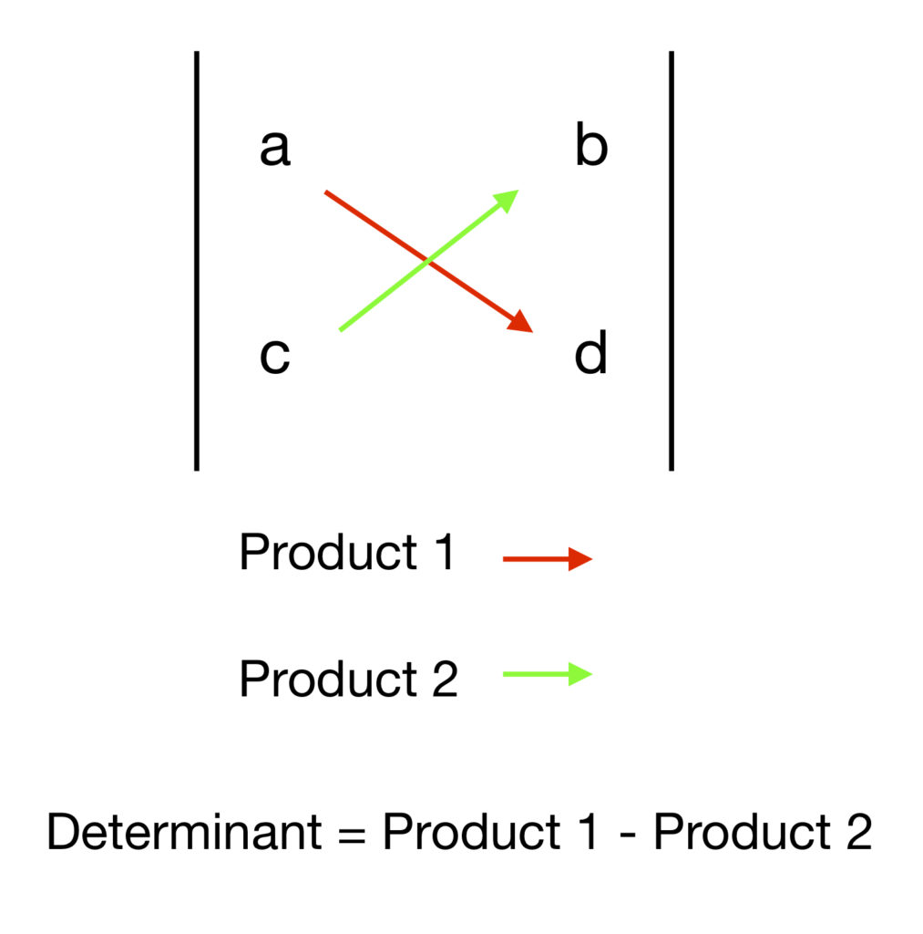
3 x 3 Matrix

Let’s start with the matrix $A=\begin{bmatrix}a_{11}&a_{12}&a_{13}\\a_{21}&a_{22}&a_{23}\\a_{11}&a_{12}&a_{13}\end{bmatrix}$

By rule 3a (linearity), it’s determinant, $\begin{vmatrix}A\end{vmatrix}$ can be broken down into the sum of three other determinants, $\begin{vmatrix}A_{11}\end{vmatrix}$ , $\begin{vmatrix}A_{12}\end{vmatrix}$ and $\begin{vmatrix}A_{13}\end{vmatrix}$ such that,

$\begin{align*}\begin{vmatrix}A\end{vmatrix}&=\begin{vmatrix}A_{11}\end{vmatrix}+\begin{vmatrix}A_{12}\end{vmatrix}+\begin{vmatrix}A_{13}\end{vmatrix}\\&=\begin{vmatrix}a_{11}&0&0\\a_{21}&a_{22}&a_{23}\\a_{11}&a_{12}&a_{13}\end{vmatrix}+\begin{vmatrix}0&a_{12}&0\\a_{21}&a_{22}&a_{23}\\a_{11}&a_{12}&a_{13}\end{vmatrix}+\begin{vmatrix}0&0&a_{13}\\a_{21}&a_{22}&a_{23}\\a_{11}&a_{12}&a_{13}\end{vmatrix}\end{align*}$

$\begin{vmatrix}A_{11}\end{vmatrix}$ , $\begin{vmatrix}A_{12}\end{vmatrix}$ and $\begin{vmatrix}A_{13}\end{vmatrix}$ can be further broken down into the sum of 9 determinants each, as shown in the following three diagrams:

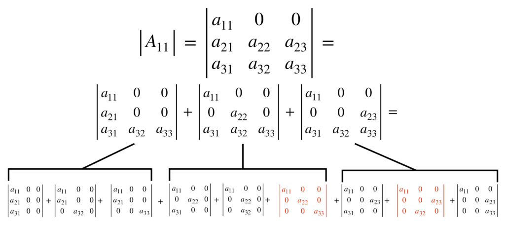
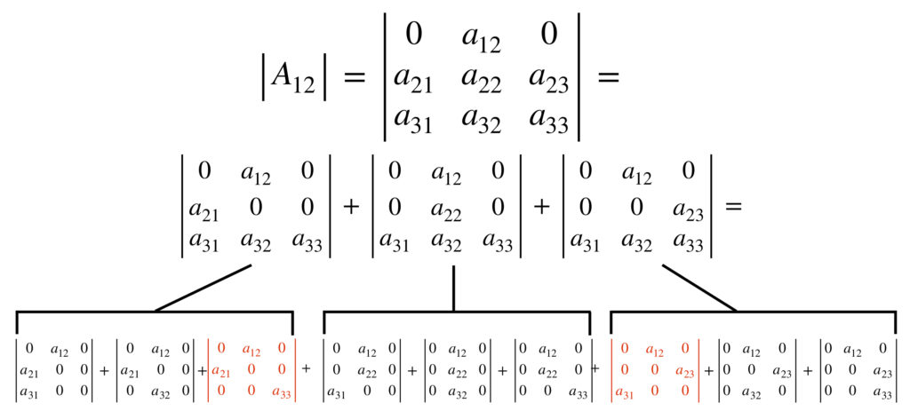
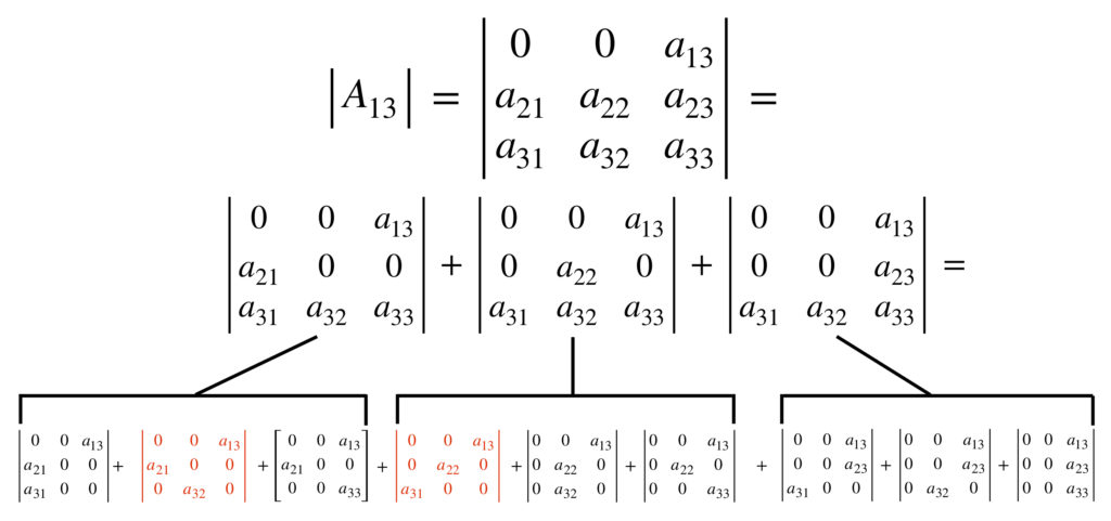
Thus, $\begin{vmatrix}A\end{vmatrix}$ can ultimately be expressed as a sum of 27 ( $=n^n=3^3=27$ ) determinants. However, by determinant property 6, if a matrix has a row of zeros, then its determinant is zero. And by property 10, $\begin{vmatrix}A\end{vmatrix}=\begin{vmatrix}A^T\end{vmatrix}$ . This means that a column of zeros in a matrix will also make its determinant zero. Or we could apply the more convoluted argument used in the proof of the 2×2 matrix formula above. Either way, from the above diagrams, it is apparent that 21 out of the 27 determinants that add up to make up $\begin{vmatrix}A\end{vmatrix}$ have at least one column of zeros. The determinants of these matrices are zero. Thus, only 6 ( $=n!=3!=3\cdot2\cdot1=6$ ) of the 27 determinants contribute to $\begin{vmatrix}A\end{vmatrix}$ .

Let’s take a look at what makes a term zero versus actually contributing to the value of the determinant. Basically, we’re trying to convert the determinants of permutation matrices into the identity matrix by row exchanges. The identity matrix has a 1 in each row and column. All the rest of the entries in the row and column that contains the 1 are zeros. Therefore, to make a row exchange or exchanges that yields the identity matrix, the permutation matrix on which the row exchange is being made must also contain only a single 1 (and all the rest zeros) in each of its rows and columns. In contrast, as stated above, if a permutation matrix contains a row or column of zeros, then its determinant is 0 and it makes no contribution to the overall determinant we are trying to calculate.

As alluded to above, for an 3 x 3 matrix, there are $3!$ determinants that contribute to the overall determinant. Why? because, as we’ve already seen, we can break the determinant of that matrix down into the sum of the products of three coefficients times a permutation matrix. If a term in that sum is to contribute to the overall determinant of the original 3×3 matrix, the permutation matrix associated with that term has to have a single one in each of its rows (or, because $\det{A}=\det{A^T}$ , its columns). Thus, if such a permutation has a 1 in column 1, there are three possible rows that such a 1 in column 1 can be positioned. For each of these resulting determinants, since row 1 is already “taken,” there are two possible rows in which the second 1 can be positioned, and that leaves one one remaining row in which the third 1 can be positioned. So for each three “subdeterminants,” there are two other configurations in which the 1’s can be positioned and still contribute to the overall determinant of the original 3 x 3 matrix; that’s $3\times2\times1=3!=6$ . This argument can be extended to the n x n case. For example, for a 4 x 4 matrix, the number of terms that such a matrix can be broken down into equals $4^4=256$ . However, the number of terms that actually contribute to the determinant is $4!=4\times3\times2\times1=24$ .

As seen in the proof of determinant property 7-using determinant property 3b-these 6 determinants can be simplified into the product of three coefficients times the determinant of a permutation of the identity matrix. This determinant can then be turned into the determinant of the identity matrix by making row exchanges. This is done because, by rule 1, the determinant of the identity matrix is 1. Multiplying the expression of the product of the three coefficients times 1 (i.e., the determinant of the identity matrix) leaves just the product of the three coefficients. However, by rule 2, the sign of the determinant changes when row exchanges are made. Thus, if an odd number of row exchanges is required to change the determinant of the permutation of the identity matrix to that of the identity matrix, then the products of coefficients must be multiplied by -1 instead of 1. If an even number of row exchanges are needed, then the coefficients are multiplied by +1.

Here are two examples:

After applying rule 3b to $\begin{vmatrix}A\end{vmatrix}$ , we get,

$\begin{array}{rcl}\begin{vmatrix}A\end{vmatrix}=\begin{vmatrix}a_{11}&a_{12}&a_{13}\\a_{21}&a_{22}&a_{23}\\a_{11}&a_{12}&a_{13}\end{vmatrix}&=&a_{11}a_{22}a_{33}\begin{vmatrix}1&0&0\\0&1&0\\0&0&1\end{vmatrix}+a_{12}a_{23}a_{31}\begin{vmatrix}0&1&0\\0&0&1\\1&0&0\end{vmatrix}+a_{13}a_{21}a_{32}\begin{vmatrix}0&0&1\\1&0&0\\0&1&0\end{vmatrix}\\&\,& +a_{11}a_{23}a_{32}\begin{vmatrix}1&0&0\\0&0&1\\0&1&0\end{vmatrix}+a_{12}a_{21}a_{33}\begin{vmatrix}0&1&0\\1&0&0\\0&0&1\end{vmatrix}+a_{13}a_{22}a_{31}\begin{vmatrix}0&0&1\\0&1&0\\1&0&0\end{vmatrix}\end{array}$

Next, perform row exchanges until each determinant in the equation above become the identity matrix. To do this, the first three determinants on the right side of the above equation require zero or two row exchanges. Thus, the product of the three coefficients in these terms are each multiplied by +1. On the other hand, the second three terms in the above equation require one row exchange. Therefore, the product of the three coefficients in these terms are each multiplied by -1. That leave us with,

$\begin{array}{rcl}\det{A}&=&a_{11}a_{22}a_{33}+a_{12}a_{23}a_{31}+a_{13}a_{21}a_{32}\\&\,&-a_{11}a_{23}a_{32}-a_{12}a_{21}a_{33}-a_{13}a_{22}a_{31}\end{array}$

which is the big formula for the determinant of a 3 x 3 matrix.

From the above considerations, we can come up with a general expression for the big formula of a square matrix of any size. Let $A$ be a square matrix with columns $(1,2,\dots,n)$ . The permutation matrices that cause terms to contribute to the overall determinant are ordered in ways that we will call $(\alpha,\beta,\dots\omega)$ where $\alpha,\beta,\dots\omega$ are unique for a given term and specify the rows in the permutation matrix where the 1’s are found.

For example, for a 3 x 3 matrix, the six possibilities for $\alpha,\beta,\gamma$ are $(123), (231), (312), (132), (213), (321)$ .

We’ll follow the nomenclature in Strang’s text and define an entity, $\det{P(\alpha\beta\gamma\,\dots\,\omega)}$ which is basically the +1 or -1 by which we multiply the product of coefficients, an entity determined by how many row exchanges it takes to change a given permutation matrix into the identity matrix.

In the case of a 3 x 3 matrix, the $\det{P}$ values for each permutation matrix are as follows:

$\det{P(1,2,3)}=+1$	$\det{P(2,3,1)}=+1$	$\det{P(3,1,2)}=+1$
$\det{P(1,3,2)}=-1$	$\det{P(2,1,3)}=-1$	$\det{P(3,2,1)}=-1$

Then, for an n x n matrix:

$\det{A}=\displaystyle\sum_\alpha^\omega\det{P(\alpha\beta\gamma\,\dots\,\omega)}a_{1\alpha}a_{2\beta}a_{3\gamma}\,\dots\,a_{n\omega}$

The cofactor formula

There are several ways to calculate the determinant of a square matrix. One that we haven’t discussed in detail is to reduce the matrix into reduced row echelon form and take the product of the diagonal elements. By property 7, this is the determinant of the matrix. A second method, which we just outlined, is the big formula. A third method, which we can derive by factoring out terms from the big formula, is the so-called cofactor method, which we present here. We’ll present the formula, then show why it makes sense. A good discussion of this topic can be found at the following source:

https://www.math.purdue.edu/files/academic/courses/2010spring/MA26200/3_3.pdf

Our ideas here will be largely taken from this source. Here goes:

Define an entity called a minor as follows:

Let $A$ be an n x n matrix. The minor, $M_{ij}$ , of an element of $A$ , $a_{ij}$ , is the determinant of the matrix obtained by deleting the $i$ th row vector and $j$ th column vector of $A$ .

So if $A=\begin{bmatrix}a_{11}&a_{12}&a_{12}\\a_{21}&a_{22}&a_{23}\\a_{31}&a_{32}&a_{33}\end{bmatrix}$

then, for example

$M_{23}=\begin{vmatrix}a_{11}&a_{12}\\a_{31}&a_{32}\end{vmatrix}\quad\text{and}\quad M_{31}=\begin{vmatrix}a_{12}&a_{13}\\a_{22}&a_{23}\end{vmatrix}$

For example, for

$A=\begin{bmatrix}a_{11}&a_{12}&a_{13}\\a_{21}&a_{22}&a_{23}\\a_{31}&a_{32}&a_{33}\end{bmatrix}$

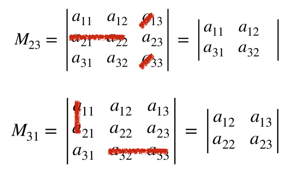
Here’s another definition:

For the same matrix, $A$ , the cofactor, $C_{ij}$ of element $a_{ij}$ , is

$C_{ij}=(-1)^{i+j}M_{ij}$

where $M_{ij}$ is the minor of $a_{ij}$ .

From the above definition, we see that the cofactor of $a_{ij}$ and the minor of $a_{ij}$ are the same if $i+j$ is even, and differ by a minus sign if $i+j$ is odd. The appropriate sign for the cofactor, $C_{ij}$ is easy to remember because it alternates in the following manner:

$\begin{vmatrix}+&-&+&-&+&\cdots\\-&+&-&+&-&\cdots\\+&-&+&-&+&\cdots\\ \vdots&\vdots&\vdots&\vdots&\vdots&\cdots\end{vmatrix}$

So for matrix $A=\begin{bmatrix}a_{11}&a_{12}&a_{13}\\a_{21}&a_{22}&a_{23}\\a_{31}&a_{32}&a_{33}\end{bmatrix}\quad C_{23}=-M_{23} \quad C_{31}=+M_{31}$

With these definitions under our belts, we are now ready to state the cofactor formula for the determinant. Here it is:

$\det{A}=a_{11}C_{11}+a_{12}C_{12}+\cdots+a_{1n}C_{1n}=\displaystyle\sum_{k=1}^n a_{1k}C_{1k}$

To see why this works, it is instructive to consider the case of a 3 x 3 matrix. Let $\begin{vmatrix}A\end{vmatrix}=\begin{vmatrix}a_{11}&a_{12}&a_{13}\\ a_{21}&a_{22}&a_{23}\\ a_{31}&a_{32}&a_{33}\\ \end{vmatrix}$

We’ve already seen that the big formula for this determinant is:

$\begin{array}{rcl}\det{A}&=&a_{11}a_{22}a_{33}+a_{12}a_{23}a_{31}+a_{13}a_{21}a_{32}\\&\,&-a_{11}a_{23}a_{32}-a_{12}a_{21}a_{33}-a_{13}a_{22}a_{31}\end{array}$

Collecting terms, we have,

$\det{A}=a_{11}(a_{22}a_{33}-a_{23}a_{32})+a_{12}(a_{23}a_{31}-a_{21}a_{33})+a_{13}(a_{21}a_{32}-a_{22}a_{31})$

The three quantities in parentheses correspond to the cofactors defined above.

If we use determinant property 3a and split $\det{A}$ into the three determinants that follow, it is easy to see how the cofactor formula comes about:

$\begin{vmatrix}A\end{vmatrix}=\begin{vmatrix}a_{11}&0&0\\ 0&a_{22}&a_{23}\\ 0&a_{32}&a_{33}\\ \end{vmatrix}+\begin{vmatrix}0&a_{12}&0\\ a_{21}&0&a_{23}\\ a_{31}&0&a_{33}\\ \end{vmatrix}+\begin{vmatrix}0&0&a_{13}\\ a_{21}&a_{22}&0\\ a_{31}&a_{32}&0\\ \end{vmatrix}$

Take the matrix that contains $a_{12}$ as the only entry in it’s first row as an example. If we cross out the row and the column that contain $a_{12}$ (i.e., row 1 and column 2), we’re left with a 2 x 2 matrix whose determinant is the minor of $a_{12}$ . If we multiply this minor by $a_{12}$ and put a minus sign in front of it (because that’s what the formula says to do), then you’ve got the $a_{12}$ -containing term that contributes to $\det{A}$ .

And if we apply the linearity properties of the determinant (i.e., rules 3a and 3b) to the matrix that contains $a_{12}$ as the only entry in it’s first row, we will obtain the same result. To see this, click on the link that follows:

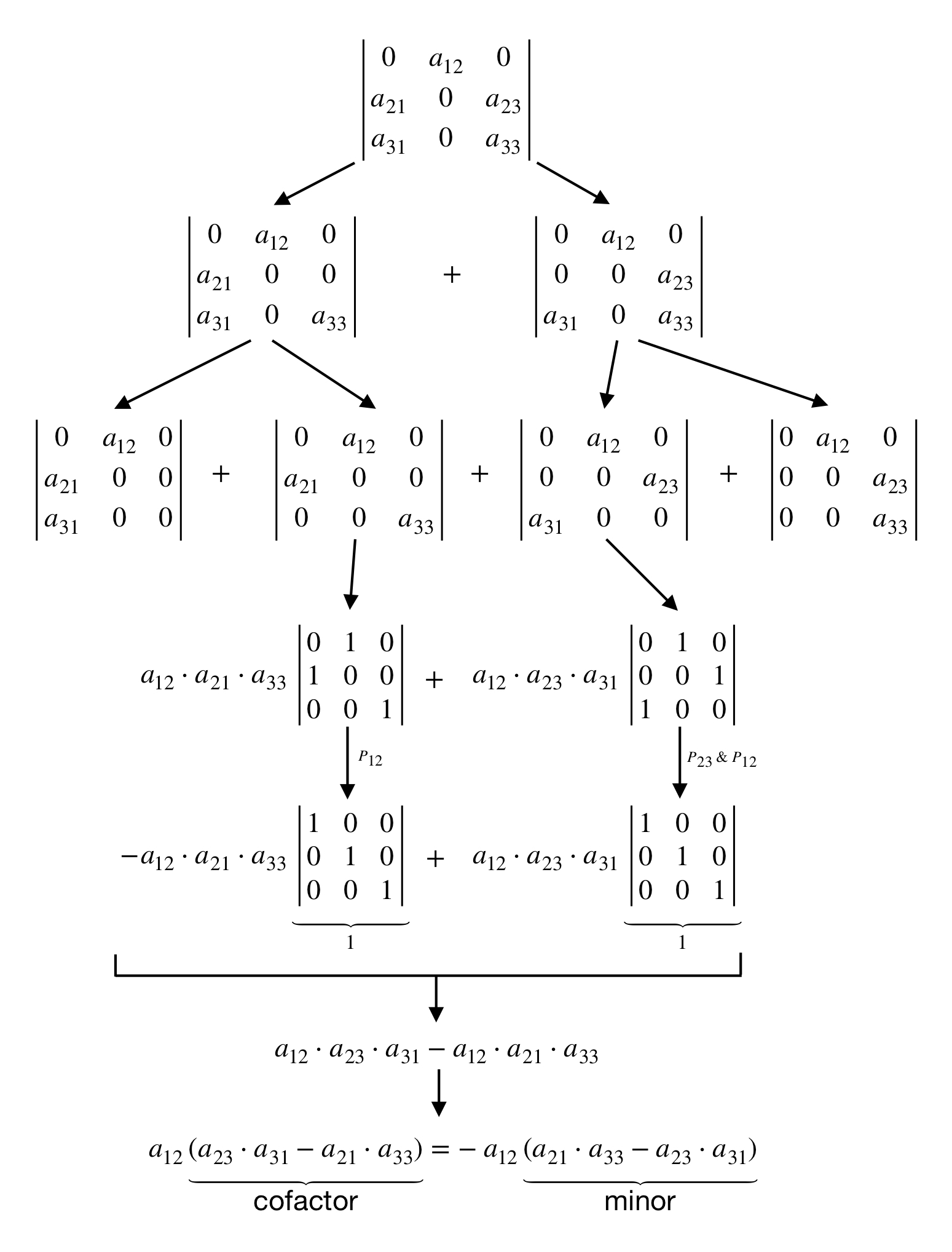
A proof of the general cofactor formula for the determinant, taken from the link from Purdue University listed above, is as follows:

For some matrix $A$ , we’ve seen that one of the ways to calculate $\det{A}$ is the big formula. We’ve also seen that we can factor out terms and the resulting rearranged expression will be equivalent to the original expression from which it came. In the example shown above, we factored out entries from the first row of the matrix. However, there’s no reason why we couldn’t factor out entries from any other row. Therefore, a general expression for such a factored expression for any row is

$\det{A}=a_{i1}X_{i1}+a_{i2}X_{i2}+\cdots+a_{in}X_{in}$

where the coefficients $X_{ij}$ contains no elements from row $i$ or column $j$ . In short, the $X_{ij}$ coefficients are terms like $(a_{21}a_{33}-a_{23}a_{31})$ noted in the example above. What we need to prove is that

$X_{ij}=C_{ij}$

where $C_{ij}$ is the cofactor of some matrix element $a_{ij}$ . Consider first the element $a_{11}$ . From the big formula, the terms of $\det{A}$ that contain $a_{11}$ are given by

$a_{11}\displaystyle\sum_\beta^\omega\det{P(1,\,\beta,\,\gamma\,\dots\,\omega)}a_{2\beta}a_{3\gamma}\,\dots\,a_{n\omega}$

Thus,

$X_{ij}=\sum_\beta^\omega\det{P(1,\,\beta,\,\gamma\,\dots\,\omega)}a_{2\beta}a_{3\gamma}\,\dots\,a_{n\omega}$

However, this summation is just the minor of $a_{11}$ (which we’ve previously called $M_{11}$ . From the cofactor formula, the first term in that formula has a positive sign. Thus, $M_{11}=C_{11}=X_{11}$ , and we have shown that the coefficient of $a_{11}$ in $\det{A}$ is , indeed, the cofactor $C_{11}$ .

Now we need to do the same for any element in $\det{A}$ . To do this, consider the generic element $a_{ij}$ . By successively interchanging adjacent rows and columns of $A$ , we can move $a_{ij}$ to the $(1,\,1)$ position without altering the relative position of the other rows and columnsmj. This creates a new matrix that we’ll call $A^\prime$ . Obtaining $A^\prime$ from $A$ requires $i$ -1 row exchanges and $j$ -1 column exchanges. Therefore, the total number of exchanges required to obtain $A^\prime$ from $A$ is $i+j-2$ . Consequently,

$\det{A}=(-1)^{i+j-2}\det{A^\prime}=(-1)^{i+j}\det{A^\prime}$

Now for the key argument:

After all the row/column exchanges, the coefficient of $a_{ij}$ in $\det{A}$ must be $(-1)^{i+j}$ times the coefficient of $a_{ij}$ in $\det{A^\prime}$
But $a_{ij}$ occurs in the $(1,\,1)$ position of $A^\prime$ . So, as we have previously shown, it coefficient in $\det{A^\prime}$ is $M^\prime_{11}$ .
Since the relative positions of the remaining rows have not changed, it follows that $M^\prime_{11}=M_{ij}$
Therefore, the coefficient of $a_{ij}$ in $\det{A^\prime}$ is $M_{ij}$ .
Consequently, the coefficient of $a_{ij}$ in $\det{A}$ is $(-1)^{i+j}M_{ij}=C_{ij}$

This argument can be expressed mathematically as follows:

$\begin{array}{rcl}X_{ij}&=&(-1)^{i+j}X^\prime_{ij}\\X^\prime_{ij}&=&M^\prime_{ij}\\M^\prime_{ij}&=&M_{ij}\\X^\prime_{ij}&=&M_{ij}\\X_{ij}&=&(-1)^{i+j}X^\prime_{ij}=(-1)^{i+j}M_{ij}\\(-1)^{i+j}M_{ij}&=&C_{ij}\end{array}$

We can apply the above argument to elements $a_{i2},\,a_{i3}\,\dots \, a_{in}$ thus establishing the cofactor expansion along any row. The result for expansion along a column follows directly since $\det{A}=\det{A^T}$

An example that illustrates the veracity of this proof comes from examining the element $a_{12}$ from the 3 x 3 matrix $A$ that we’ve working with before. Click on the button below to see this proof.

In the future, perhaps I will provide an example here, on this page, of calculating an n x n matrix using the cofactor expansion. However, for now, in the interest of time, I will simply provide a link to a video from Khan Academy that provides such an example. The video includes calculation of the determinant of a 4 x 4 matrix at about the 10 minute make. Here is the link:

Cofactor Expansion Example

Just a final word regarding the calculation of the determinant. When evaluating a determinant, it is generally most efficient to perform row/column operations (multiplication/addition and exchanges) until all but one (or few) of the terms in a row/column are zero, then apply the cofactor formula. In this way, since most of the $a_{ij}$ terms are zero, only one or a few terms actually need to be evaluated.

Geometric interpretation of the determinant

Like matrix multiplication, looking at determinants from the point of view of linear transformations provides a geometric interpretation that further our understanding. In short, the determinant works as a scaling factor.

Recall that 1) a matrix creates a linear transformation that changes the length of basis vectors (which, for example in 2D, we called $\hat{i}$ and $\hat{j}$ ) and 2) the length of basis vectors determines the size of units that determine area in 2D, and unit boxes that determine volume in 3D. Therefore, matrices determine the size of units of area and volume in 2D and 3D, respectively.

Consider the 2D case. In the run-of-the-mill Cartesian coordinate system that we’re most familiar with, $\hat{i}=\begin{bmatrix}1\\0\end{bmatrix}$ and $\hat{j}=\begin{bmatrix}0\\1\end{bmatrix}$ . Next extend a perpendicular line in the $+y$ from the tip of $\hat{i}$ and a perpendicular line in the $+x$ direction from $\hat{j}$ . They intersect at the point $(1, 1)$ to make a polygon (in this case, a square) the basic unit of area in the Cartesian coordinate system. The matrix that creates this situation is $\begin{bmatrix}1&0\\0&1\end{bmatrix}$ . A 2 x 2 polygon in this coordinate system, then, has an area of 4 square units (of whatever unit of length we may be using). This is depicted in the following diagram:

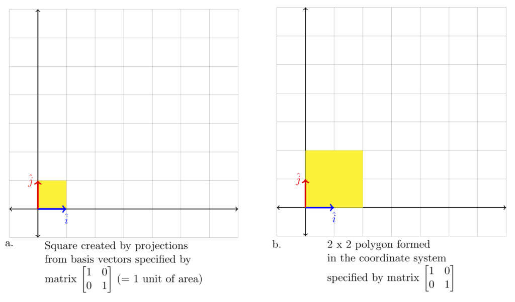
Now consider what happens if we use the matrix $\begin{bmatrix}3&1\\1&2\end{bmatrix}$ to create a linear transformation. This matrix changes $\hat{i}$ from $\begin{bmatrix}1\\0\end{bmatrix}$ to $\begin{bmatrix}3\\1\end{bmatrix}$ and $\hat{j}$ from $\begin{bmatrix}0\\1\end{bmatrix}$ to $\begin{bmatrix}1\\2\end{bmatrix}$ , forming a new coordinate system. If we perform an operation similar to what we did in the Cartesian coordinate situation (project a vector parallel to $\hat{i}$ from the end of $\hat{j}$ ; project a vector parallel to $\hat{j}$ from the end of $\hat{i}$ ), we get a polygon that represents 1 unit of area in the new coordinate system. This is depicted in the following diagram. Also depicted is a 2 x 2 polygon (in this case, a parallelogram) in this new coordinate system.

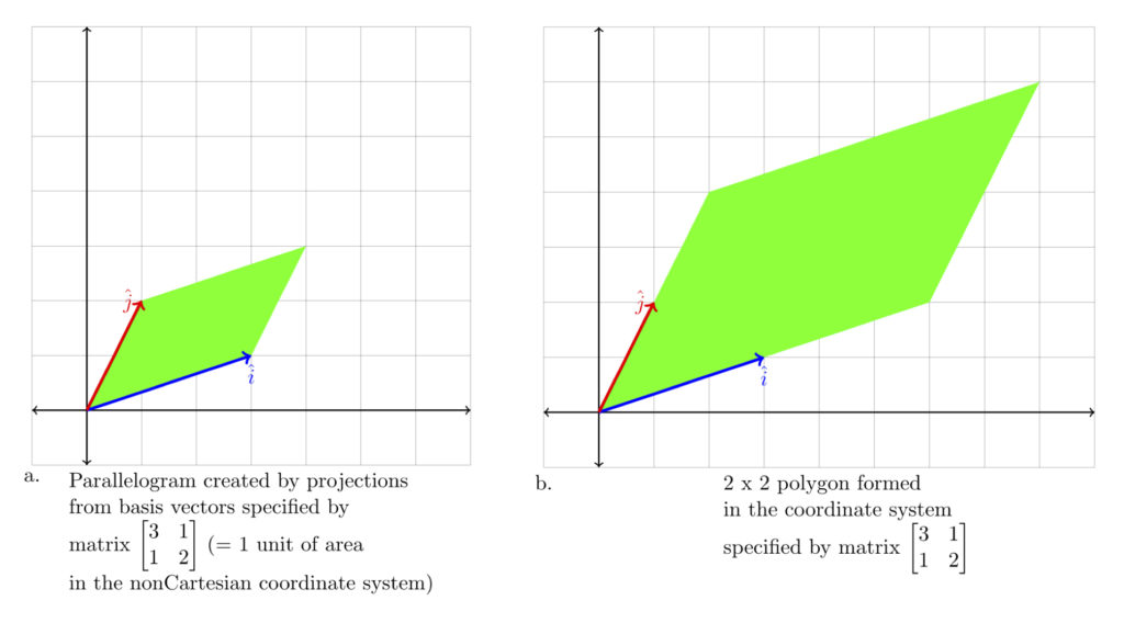
Note that the parallelogram that represents the unit of area in the new coordinate system looks bigger than that in the Cartesian coordinate system. How much bigger? Well, we can actually derive a formula for this unit area. We’ll derive the general formula first, then determine what the unit area is in the above specific case.

Rendered by QuickLaTeX.com

Our goal is to find the area of the green parallelogram depicted above. To accomplish this, we do the following:

Drop a perpendicular from the tip of $\hat{j}$ to $\hat{i}$ ; call it $\hat{h}$ .
Draw a vector along $\hat{i}$ from the origin to the point where $\hat{h}$ intersects $\hat{i}$ ; call it $\hat{p}$ (for projection; $\hat{p}$ is the projection of $\hat{j}$ onto $\hat{i}$ ).
Since $\hat{p}$ is on $\hat{i}$ , we can express $\hat{p}$ as a multiple of $\hat{i}$ , $\hat{p}=x\hat{i}$ where $x$ is some constant (from the above diagram, it looks like it’s a fraction).
Note that $\hat{h}=\hat{j}-\hat{p}$ , and based on what we just said, $\hat{h}=\hat{j}-x\hat{i}$ .
Since $\hat{h}$ is perpendicular to $\hat{i}$ , the dot product $\hat{i}\cdot\hat{h}=0 \Rightarrow \hat{i}\cdot(\hat{j}-x\hat{i})=0$

Now we need to do some algebra:

$\begin{array}{rcl} \hat{i}\cdot(\hat{j}-x\hat{i})&=&0\\ \hat{i} \cdot \hat{j} - x\hat{i} \cdot \hat{i} &=& 0 \\ \hat{i} \cdot \hat{j} &=& x\hat{i} \cdot \hat{i} \\ x &=& \frac{\hat{i} \cdot \hat{j}}{\hat{i} \cdot \hat{i}} \end{array}$

So,

$\hat{p}=x\hat{i}=(\frac{\hat{i} \cdot \hat{j}}{\hat{i} \cdot \hat{i}})\hat{i}$

Now we’re ready to find the area of the green parallelogram.

The area of that parallelogram, $A$ , equals its base times its height: $A=BH$ .
The base, $B$ , equals the length of $\hat{i}\,(=\lvert \hat{i} \rvert)$ ; $(\lvert \hat{i} \rvert)=\sqrt{\hat{i} \cdot \hat{i}}$ .
The height, $H=\hat{h}^2$ ; It is unknown but can be found by the Pythagorean theorem:

$\begin{array}{rcl}\lvert\hat{j}\rvert^2&=&\lvert\hat{h}\rvert^2 + \lvert\hat{p}\rvert^2\\ \lvert H \rvert^2&=&\lvert\hat{j}\rvert^2 - \lvert\hat{p}\rvert^2 \\ &=& \hat{j} \cdot \hat{j} - \lvert (\frac{\hat{i} \cdot \hat{j}}{\hat{i} \cdot \hat{i}})\hat{i} \rvert^2 \\ &=& \hat{j} \cdot \hat{j} - \left[\frac{\hat{i} \cdot \hat{j}}{\hat{i} \cdot \hat{i}}\hat{i} \cdot \frac{\hat{i} \cdot \hat{j}}{\hat{i} \cdot \hat{i}}\hat{i}\right] \\ &=& \hat{j} \cdot \hat{j} - \left[\frac{(\hat{i} \cdot \hat{j})(\hat{i} \cdot \hat{j})}{(\hat{i} \cdot \hat{i})(\hat{i} \cdot \hat{i})} \hat{i} \cdot \hat{i}\right] \\ &=& \hat{j} \cdot \hat{j} - \frac{(\hat{i} \cdot \hat{j})^2}{\hat{i} \cdot \hat{i}} \end{array}$

We said that $A=BH$ . That means that $A^2=B^2H^2$ . Since $B=\sqrt{\hat{i} \cdot \hat{i}}$ , $B^2=\hat{i} \cdot \hat{i}$ . That gives us

$\begin{array}{rcl}A^2&=&\hat{i} \cdot \hat{i}\left[ \hat{j} \cdot \hat{j} - \frac{(\hat{i} \cdot \hat{j})^2}{\hat{i} \cdot \hat{i}} \right] \\ &=& (\hat{i} \cdot \hat{i})(\hat{j} \cdot \hat{j}) - (\hat{i} \cdot \hat{j})^2 \end{array}$

Next, recall that it’s matrices that bring about linear transformations and specify $\hat{i}$ and $\hat{j}$ . Let’s consider the generic 2 x 2 matrix $\begin{bmatrix}a&b\\c&d\end{bmatrix}$ . This matrix makes $\hat{i}=\begin{bmatrix}a\\c\end{bmatrix}$ and $\hat{j}=\begin{bmatrix}b\\d\end{bmatrix}$ .

Let’s substitute these values into the equation above:

$\begin{array}{rcl} \hat{i} \cdot \hat{i} &=& \begin{bmatrix}a&c\end{bmatrix}\begin{bmatrix}a\\c\end{bmatrix}=a^2 + c^2 \\ \hat{j} \cdot \hat{j} &=& \begin{bmatrix}b&d\end{bmatrix}\begin{bmatrix}b\\d\end{bmatrix}=b^2 + d^2 \\ \hat{i} \cdot \hat{j} &=& \begin{bmatrix}a&c\end{bmatrix}\begin{bmatrix}b\\d\end{bmatrix}=ab + bd \end{array}$

That means that

$\begin{array}{rcl} A^2&=&(a^2+c^2)(b^2+d^2)-(ab + cd)^2 \\ &=& a^2b^2+a^2d^2+c^2b^2+c^2d^2-(a^2b^2+2abcd+c^2d^2) \\ &=& \cancel{a^2b^2}+a^2d^2+c^2b^2+\cancel{c^2d^2}- \cancel{a^2b^2}-2abcd-\cancel{c^2d^2} \\ &=& a^2d^2-2abcd+c^2b^2 \\ &=& (ad-bc)^2 \\ A &=& ad-bc\end{array}$

But $ad-bc$ is the determinant of the matrix $\begin{bmatrix}a&b\\c&d\end{bmatrix}$ . Therefore,

The area of the parallelogram formed from the basis vectors specified by a 2 x 2 matrix is given by the determinant of that matrix.

Rendered by QuickLaTeX.com

$\begin{array}{rcl}\text{Area }&=&(a+b)(c+d)-2(\frac{ac}2)-2(\frac{bd}2)-2bc\\&=& \cancel{ac}+ad+bc+\cancel{bd}-\cancel{ac}-\cancel{bd}-2bc \\ &=& ad-bc = \begin{vmatrix}a&b\\c&d\end{vmatrix} \end{array}$

Just as the basis vectors specified by a 2 x 2 matrix can be projected to form a parollelogram, the basis vectors specified by a 3 x 3 matrix can be projected to form a parallelepiped. And by similar arguments to those described for the 2 x 2 matrix, the determinant of a 3 x 3 matrix is the volume of the parallelepiped it forms.

A generic proof that the determinant of a matrix is the “volume” (or analog of volume) of a “parallelepiped” (or, more generally, geometric object) is taken from Strang’s textbook and the following link:

https://textbooks.math.gatech.edu/ila/determinants-volumes.html

Let’s start by defining the generic version of a parallelepiped. The parallelepiped determined by $n$ vectors $v_1,\,v_2\,\dots,\,v_n$ in $\mathbf{R^n}$ is the subset

(1) $\begin{equation*} P=\lbrace a_1\vec{v}_1+a_2\vec{v}_2+\dots+a_n\vec{v}_n\,|\,0\leq a_1,a_2,\dots,a_n \leq 1 \rbrace \end{equation*}$

In other words, a parallelepiped is the set of all linear combinations of $n$ vectors with coefficients from 0 through 1. So the length of the vectors we’re adding together are all $\leq 1$ times (i.e., they are a fraction of) the $\vec{v}_1,\,\vec{v}_2\,\dots,\,\vec{v}_n$ vectors that they are multiplying. This puts a limit on the length of the vectors that can be added together. If we let the tip of each of these linear combinations be represented by a point, these points will all be confined to locations on or within the parallelepiped specified by the $n$ vectors we are considering.

For example, take a parallelogram specified by the vectors $\vec{v}_1$ and $\vec{v}_2$ :

Rendered by QuickLaTeX.com

If we add $\vec{v}_2$ to every point along $\vec{v}_1$ , we get the upper margin of the parallelogram. If we add $\vec{v}_2$ to $\vec{v}_1$ , we get the right-hand margin. If we multiply each of an infinite number of coefficients, $a$ times $\vec{v}_2$ , we get all of the points along the left-hand margin. And if we multiply an infinite number of coefficients, $a$ times $\vec{v}_1$ , we get all of the points along the bottom margin of the parallelogram. If we create points from all of the other linear combinations we can make from coefficients $\leq 1$ times $\vec{v}_1$ and $\vec{v}_2$ , we get the inside of the parallelogram.

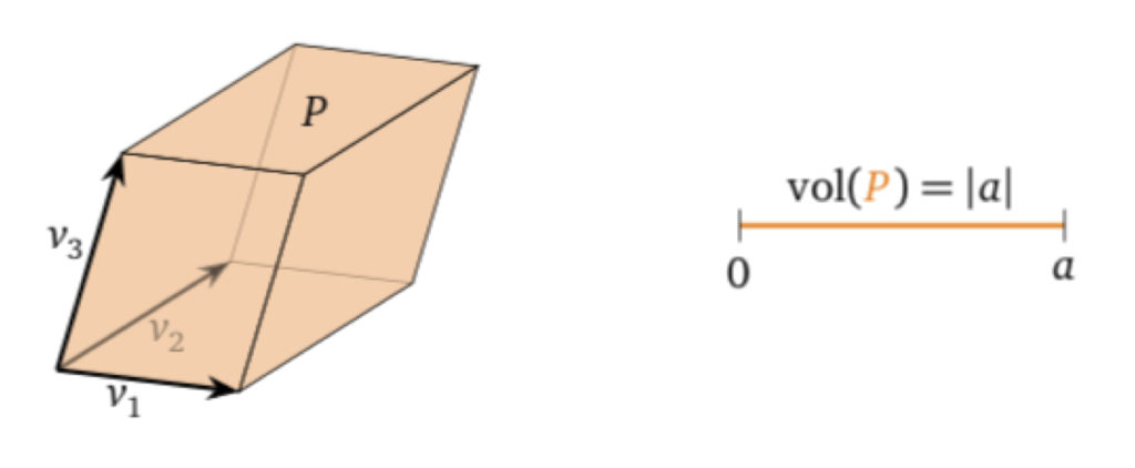
By the above argument, we can see how 3 vectors can be associated with a 3D parallelepiped (on the left in the above diagram). On the other hand, a single vector is associated with a “1D parallelepiped,” better known as a line, and its volume-analogue is its length (as shown in the figure on the right). Similar arguments can also be applied larger numbers of vectors creating higher dimensional objects (although such objects are difficult to visualize and diagram).

From this, the question arises: when does a parallelepiped formed in the way described above have zero volume? Answer: when it is squashed to a lower dimension (e.g., two vectors that form a line, three vectors that form a plane). And when does this occur? When one or more of the vectors $\vec{v}_1,\,\vec{v}_2\,\dots,\,\vec{v}_n$ are linearly dependent (i.e., are linear combinations of other vectors in the set). This is shown in the diagram below:

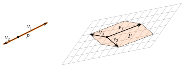
Now if we have a matrix, $A$ , with two rows that are multiples of each other, if we multiply one of these rows by the correct factor, and subtract it from its linearly dependent counterpart, we create a new matrix, $A^\prime$ , with a row of zeros. But by determinant property 6, if a matrix has a row of zeros, then its determinant is zero. Furthermore, since we created $A^\prime$ by subtracting a multiple of one row from another, by determinant property 5, $\det{A}=\det{A^\prime}$ . And since $\det{A^\prime}=0$ , $\det{A}$ also equals zero. This leads us to the conclusion that, if a matrix has two (or more) rows that are linear dependent (i.e., are linear combinations of each other), then its determinant is zero. And because determinant property 10 says that $\det{A}=\det{A^T}$ , the same applies if two or more columns of a matrix are linearly dependent.

So here’s the punchline:

A parallelepiped formed from a matrix with columns $\vec{v}_1,\,\vec{v}_2\,\dots,\,\vec{v}_n$ has a volume of zero if and only if it has linearly dependent rows or columns.
If a matrix has linearly dependent rows or columns, then its determinant is zero.

Therefore, a parallelepiped formed from the columns of a matrix, $\vec{v}_1,\,\vec{v}_2\,\dots,\,\vec{v}_n$ , has zero volume if and only if the determinant of that matrix is zero.

But this is only the beginning of the story. It turns out that the volume of such a parallelepiped is always a determinant. Specifically,

Let $\vec{v}_1,\,\vec{v}_2\,\dots,\,\vec{v}_n$ be vectors in $\mathbf{R^n}$ , let $P$ be the parallelepiped determined by these vectors, and let $A$ be the matrix with rows $\vec{v}_1,\,\vec{v}_2\,\dots,\,\vec{v}_n$ . Then the absolute value of the determinant of $A$ is the volume of $P$ :

$\lvert \det{A} \rvert = \text{vol}(P)$

To prove this, we’ll prove that $\text{vol}(P)$ follows properties 1-3 of the determinant.

Property 1: The determinant of the identity matrix, $I_n$ , is equal to 1.

If the number of dimensions is one, and the matrix $A=1$ , then its “volume-analogue” (= its length) equals 1 and so does $\det{A}$ .
If we’re dealing with a 2-dimensional space, the area of such a space is the unit square which equals 1. In this case, the matrix $A$ would equal $I$ and $\det{A}$ , like the area, would also be 1.
If we’re dealing with a 3D space, the volume would be the unit cube which has volume 1. In this case, the matrix $A$ would equal $I_3$ and $\det{A}$ , like the area, would also be 1.
If $n > 3$ , then the volume-analogue is still 1 unit. The matrix associated with this space is $A=I_n$ . The determinant of that matrix, like any version of the identity matrix, is still 1.

Property 2: The determinant changes sign when two rows are exchanged.

However, a corollary to this property is that, although the sign of the determinant changes, its absolute value remains unchanged. When we swap rows, we just change the order of the rows in the matrix. When we make, for example, a parallelogram out of those rows, we change the orientation of the parallelogram. However, the angle between the vectors and the vector magnitudes remain the same. Therefore, the area of the new parallelogram remains the same. The same argument applies to other parallelepipeds as well. The following is an example of this in two dimensions:

Rendered by QuickLaTeX.com

The area of this parallelogram equals base times height: $\text{Area}=BH$ .
$B$ equals the length of $\vec{v_1}$ , $\lvert \vec{v_1} \rvert=\sqrt{3^2 + 1^2}=\sqrt{10}$ .
$H=\lvert \vec{v_2} \rvert \sin \theta \text{ where } \theta = \text{ the angle between } \vec{v_1} \text{ and } \vec{v_2}$ .
$\cos \theta = \frac {\vec{v_1} \cdot \vec{v_2}}{\lvert \vec{v_1} \rvert \lvert \vec{v_2} \rvert}=\frac{(3)(1)+(1)(2)}{\sqrt{3^2 + 1^2} \sqrt{1^2 + 2^2} }=\frac{5}{\sqrt{10}\sqrt{5}}=\frac{5}{\sqrt{50}}=\frac{5}{\sqrt{2 \cdot 25}}=\frac{5}{5\sqrt{2}}=\frac{1}{\sqrt{2}}$ .
$\arccos{\frac{1}{\sqrt{2}}=45^\circ$
$H=\lvert \vec{v_2} \rvert \sin\theta=\sqrt{1^2+2^2}\sin 45^\circ=\sqrt{5}{\frac{1}{\sqrt{2}}$
So $\text{Area}=BH=\frac{\sqrt{10}\sqrt{5}}{\sqrt{2}}=\frac{\sqrt{50}}{\sqrt{2}}=\frac{\sqrt{25}\cancel{\sqrt{2}}}{\cancel{\sqrt{2}}}=5$

Rendered by QuickLaTeX.com

The area of the above parallelogram equals base times height: $\text{Area}=BH$ .
$B$ equals the length of $\vec{v_1}$ , $\lvert \vec{v_1} \rvert=\sqrt{3^2 + 1^2}=\sqrt{10}$ .
$H=\lvert \vec{v_2} \rvert \sin \theta \text{ where } \theta = \text{ the angle between } \vec{v_1} \text{ and } \vec{v_2}$ .
$\cos \theta = \frac {\vec{v_1} \cdot \vec{v_2}}{\lvert \vec{v_1} \rvert \lvert \vec{v_2} \rvert}=\frac{(1)(2)+(3)(1)}{\sqrt{1^2 + 3^2} \sqrt{2^2 + 1^2} }=\frac{5}{\sqrt{10}\sqrt{5}}=\frac{5}{\sqrt{50}}=\frac{5}{\sqrt{2 \cdot 25}}=\frac{5}{5\sqrt{2}}=\frac{1}{\sqrt{2}}$ .
$\arccos{\frac{1}{\sqrt{2}}=45^\circ$
$H=\lvert \vec{v_2} \rvert \sin\theta=\sqrt{1^2+2^2}\sin 45^\circ=\sqrt{5}{\frac{1}{\sqrt{2}}$
So $\text{Area}=BH=\frac{\sqrt{10}\sqrt{5}}{\sqrt{2}}=\frac{\sqrt{50}}{\sqrt{2}}=\frac{\sqrt{25}\cancel{\sqrt{2}}}{\cancel{\sqrt{2}}}=5$

So we can see that the areas of these two parallelograms-formed from matrices whose rows have been swapped-are equal. And since, when we apply row swaps to higher dimensional matrices, we make them one at a time. Geometrically, that correlates with swapping vectors on a single “face” of the higher dimensional object. And that “face” is just a 2D parallelogram. So the argument we just went through for parallelograms applies exactly to the row swaps we make in the higher dimensional object. When we make such a row swap in a higher dimensional geometric object, the area of the object, after a swap, remains the same.

You may have noticed that the determinants of the row-swapped matrices that were used to construct the two parallelograms above actually have opposites signs:

$\det{A}=\begin{vmatrix}3&1\\1&2\end{vmatrix}=3\cdot2-1\cdot1=5 \quad \quad \det{A^\prime}=\begin{vmatrix}1&2\\3&1\end{vmatrix}=1\cdot1-3\cdot2=-5$

However, this doesn’t contradict the theorem we are trying to prove,

$\lvert \det{A} \rvert = \text{vol}(P)$

since

$\lvert \det{A} \rvert=\lvert 5 \rvert=\lvert \det{A^\prime} \rvert=\lvert -5 \rvert=5=\text{vol}(P)$

However, there is a geometric analogue for negative area. It involves application of the so-called right hand rule:

Put your hand on $\vec{v_1}$ .
Curl your fingers toward $\vec{v_2}$ and stick your thumb up.
If your thumb points out of the paper (or screen) toward you, it represents positive area.
If your thumb points into the paper (or screen) away from you, it represents negative area.
For 3D volumes
- Position your hand on $\vec{v_1}$ and $\vec{v_2}$ as in the 2D case
- If the component of the third vector that determines the volume points in the same direction as your thumb, the volume is positive.
- If the component of the third vector that determines the volume points in the opposite direction of your thumb, the volume is negative.
Visualization is difficult when $n>3$ .

Property 3a: If a row from a matrix, $B$ , is added to one of the rows of a matrix, $A$ , that is the same as $B$ except for the row to which the row from $B$ is added, the determinant of the resulting matrix, $A^\prime$ , is the sum of the determinant of $A$ plus the determinant of $B$ :

$\underbrace{\begin{vmatrix} a+a^\prime&b+b^\prime\\c&d \end{vmatrix}}_{A^\prime}=\underbrace{\begin{vmatrix} a&b\\c&d \end{vmatrix}}_{A}+\underbrace{\begin{vmatrix} a^\prime&b^\prime\\c&d \end{vmatrix}}_{B}$

The geometric analogue to this is:

$\text{Area}_{P_{A^\prime}}=\text{Area}_{P_A}+\text{Area}_{P_B}$

To illustrate this, we’ll expand the example we’ve been using, using numbers rather than variables to make visualization easier. Specifically,

$\text{Area}_{P_A}$ is the parallelogram constructed from $A=\begin{bmatrix}3&1\\1&2\end{bmatrix}$
$\text{Area}_{P_B}$ is the parallelogram constructed from $B=\begin{bmatrix}1&1\\1&2\end{bmatrix}$
is the parallelogram constructed when row 1 of is added to row 1 of :
- $A^\prime=\begin{bmatrix}3+1&1+1\\1&2\end{bmatrix}=\begin{bmatrix}4&2\\1&2\end{bmatrix}$

Rendered by QuickLaTeX.com

So,

$\underbrace{6}_{\text{Area}_{P_{A^\prime}}}=\underbrace{5}_{\text{Area}_{P_A}}+\underbrace{1}_{\text{Area}_{P_{B}}$

The areas of the parallelograms demonstrate the same addition property that the determinant does:

$\begin{array}{rcl} \det{P_{A^\prime}}&=&\det{P_{A}}+\det{P_{B}}\\ \begin{vmatrix}4&2\\1&2\end{vmatrix}&=&\begin{vmatrix}3&1\\1&2\end{vmatrix}+\begin{vmatrix}1&1\\1&2\end{vmatrix}\\ (4)(2)-(1)(2)&=&\left[(3)(2)-(1)(1)\right]+\left[(1)(2)-(1)(1)\right]\\ (8-2)&=&(6-1)+(2-1)\\ 6&=&5+1 \end{array}$

And as we discussed above, when we add a row to a matrix that determines a parallelepiped in a higher dimension, we are performing this operation on one “face” (or side). Of course, one face or side is a parallelogram, and we just proved that the area of a parallelogram follows determinant property 3a, so the “volume” of the parallelepiped must also follow determinant property 3a.

Property 3b: If we multiply a row of a matrix by some constant, then the determinant of the new matrix so created equals the determinant of the original matrix times the constant.

In equation format:

$\begin{vmatrix} a\cdot t&b\cdot t\\c&d \end{vmatrix}=t\begin{vmatrix} a&b\\c&d \end{vmatrix}$

What we want to prove is that, if we

make a parallelogram, $P_A$ from matrix $A$
multiply the second row of $P_A$ by a constant, $t$ to get a new matrix, $P_{A^\prime}$
make a parallelogram from $P_{A^\prime}$

Then the area of $P_{A^\prime}$ , $\text{Area}_P_{A^\prime}$ , equals $t$ times the area of $P_A$ ( $\text{Area}_P_A$ ):

$\text{Area}_P_{A^\prime}=t\text{Area}_P_A$

For ease of visualization, let’s prove this using numbers instead of variables, like we did in the last case. Specifically, we’ll multiply a row of the matrix $A=\begin{bmatrix} 3&1\\1&2\end{bmatrix}$ by $t=2$ , form a parallelogram from that matrix and see what happens. Since we can multiply any row of a matrix and get the same result, let’s multiply the second row of $A$ by 2. Why the second row? Simply so the resulting matrix fits on our page.

When we do this, we get:

$\begin{bmatrix} 3&1\\1\cdot 2&2\cdot 2\end{bmatrix}=\begin{bmatrix} 3&1\\2&4\end{bmatrix}=A^\prime$

Next, we make a parallelogram, like we have been doing, from the columns of $\begin{bmatrix} 3&1\\2&4\end{bmatrix}$ . We have $\vec{a_1}=\begin{bmatrix}3\\2\end{bmatrix}$ and $\vec{a_2}=\begin{bmatrix}1\\4\end{bmatrix}$ :

Rendered by QuickLaTeX.com

$\begin{array}{rcl}\text{Area}_{P_A^\prime}&=&BH \\ B&=&\lvert\vec{a^_1}\rvert=\sqrt{3^2+2^2}=\sqrt{13} \\ H&=&\lvert \vec{a_2} \rvert \sin{\theta}\quad \theta=\sphericalangle \text{ btwn } \vec{a_1} \text{ and } \vec{a_2}\\ \cos \theta &=& \frac {\vec{a_1} \cdot \vec{a_2}}{\lvert \vec{a_1} \rvert \lvert \vec{a_2} \rvert}=\frac{(3)(1)+(2)(4)}{\sqrt{3^2 + 2^2} \sqrt{1^2 + 4^2} }=\frac{11}{\sqrt{13}\sqrt{17}}\\ 11^2+x^2&=&(\sqrt{13}\sqrt{17})^2=221 \text{ by Pythagorean theorem}\\121+x^2&=&221\\ x^2&=&100\text{; }\quad x=10\\ \sin\frac{11}{\sqrt{13}\sqrt{17}} &=& \frac{\text{opposite}}{\text{hypotenuse}} =\frac{10}{\sqrt{13}\sqrt{17}}\\H&=&\cancel{\sqrt{17}}\frac{10}{\sqrt{13}\cancel{\sqrt{17}}}=\frac{10}{\sqrt{13}}\\ \text{Area}_{P_A^\prime}&=&BH=\cancel{\sqrt{13}}\frac{10}{\cancel{\sqrt{13}}}\\ \text{Area}_{P_A^\prime}&=&10 \end{array}$

We set out to prove that $\text{Area}_P_{A^\prime}=t\text{Area}_P_A$ . From our previous calculations, $\text{Area}_{P_A}=5$ . From the calculation we just performed, $\text{Area}_P_{A^\prime}=10$ . Then

$\underbrace{10}_{\text{Area}_P_{A^\prime}}=\underbrace{2}_{t}\times\underbrace{5}_{\text{Area}_P_A}$

The areas of the parallelograms demonstrate the same multiplication property that the determinant does:

$\begin{array}{rcl}\det{A^\prime}&=&2\det{A}\\ \begin{vmatrix}3&1\\2&4\end{vmatrix}&=&2\begin{vmatrix}3&1\\1&2\end{vmatrix}\\ (3)(4)-(2)(1)&=&2\left[ (3)(2)-(1)(1) \right]\\ 12-2&=&2(6-1)\\ 10&=&2\times 5 \end{array}$

This is what we sought to prove.

And similar to what we’ve argued before, when we multiply a row to a matrix that determines a parallelepiped in a higher dimension, we are performing this operation on one “face” (or side). Of course, one face or side is a parallelogram, and we just proved that the area of a parallelogram follows determinant property 3b, so the “volume” of parallelepipeds, in general, must also follow determinant property 3b.

Uses of the determinant

There are several uses of the determinant. Here are three of the most important.

Finding the inverse of a matrix

The first use of the determinant that we will discuss is finding the inverse of a matrix. The formula used to do this is:

$A^-1=\frac{C^T}{\det{A}}$ where

$A^-1$ is the inverse of a matrix, $A$
$\det{A}$ is the determinant of $A$
$C^T$ is the transverse of a matrix of cofactors for each term in $A$

Following the arguments laid out it Strang’s textbook, we will derive this formula in two steps. The first step involves describing and deriving Cramer’s rule.

Cramer’s rule

Cramer’s rule, ultimately, is a method of solving the matrix equation $A\vec{x}=\vec{b}$ , albeit a tedious one. However, it’s great for seeing where the formula for finding the inverse of a matrix using the determinant comes from.

. To do this, we start with this equation:

$\begin{bmatrix}a_{11}&a_{12}&a_{13}\\a_{21}&a_{22}&a_{23}\\a_{31}&a_{32}&a_{33}\end{bmatrix}\begin{bmatrix}1&0&0\\0&1&0\\0&0&1\end{bmatrix}=\begin{bmatrix}a_{11}&a_{12}&a_{13}\\a_{21}&a_{22}&a_{23}\\a_{31}&a_{32}&a_{33}\end{bmatrix}$

Make column 1 of the identity matrix in the above equation the vector, $\vec{x}$ that we want to find. Multiply that resulting matrix with matrix $A$ . We get a matrix that is the same as $A$ except that its first column is the vector $\vec{b}$ (i.e., the “answer” to the equation $A\vec{x}=\vec{b}$ that we want to solve):

$\begin{bmatrix}a_{11}&a_{12}&a_{13}\\a_{21}&a_{22}&a_{23}\\a_{31}&a_{32}&a_{33}\end{bmatrix}\begin{bmatrix}x_1&0&0\\x_2&1&0\\x_3&0&1\end{bmatrix}=\begin{bmatrix}b_1&a_{12}&a_{13}\\b_2&a_{22}&a_{23}\\b_3&a_{32}&a_{33}\end{bmatrix}=B_1$

Now take the determinant of the three matrices. We have:

$(\det{A})(x_1)=\det{B_1}\quad x_1=\frac{\det{B_1}}{\det{A}}$

If you’re wondering why $\begin{vmatrix}x_1&0&0\\x_2&1&0\\x_3&0&1\end{vmatrix}=x_1$ , click .

To find $x_2$ , we put $\vec{x}$ into the second column of the identity matrix, multiply, then take the determinant of the three matrices:

$\begin{bmatrix}a_{11}&a_{12}&a_{13}\\a_{21}&a_{22}&a_{23}\\a_{31}&a_{32}&a_{33}\end{bmatrix}\begin{bmatrix}1&x_1&0\\0&x_2&0\\0&x_3&1\end{bmatrix}=\begin{bmatrix}a_{11}&b_1&a_{13}\\a_{21}&b_2&a_{23}\\a_{31}&b_3&a_{33}\end{bmatrix}=B_2$

$(\det{A})(x_2)=\det{B_2}\quad x_2=\frac{\det{B_2}}{\det{A}}$

To find $x_3$ , we put $\vec{x}$ into the third column of the identity matrix, multiply, then take the determinant of the three matrices:

$\begin{bmatrix}a_{11}&a_{12}&a_{13}\\a_{21}&a_{22}&a_{23}\\a_{31}&a_{32}&a_{33}\end{bmatrix}\begin{bmatrix}1&0&x_1\\0&1&x_2\\0&0&x_3\end{bmatrix}=\begin{bmatrix}a_{11}&a_{12}&b_1\\a_{21}&a_{22}&b_2\\a_{31}&a_{33}&b_3\end{bmatrix}=B_3$

$(\det{A})(x_3)=\det{B_3}\quad x_3=\frac{\det{B_3}}{\det{A}}$

Thus,

$x_1=\frac{\det{B_1}}{\det{A}}\quad x_2=\frac{\det{B_2}}{\det{A}}\quad x_3=\frac{\det{B_3}}{\det{A}}$

Proof

So we’ve solved our equation $A\vec{x}=\vec{b}$ . Since the columns of a matrix are, themselves, vectors, we could perform matrix multiplication by applying Cramer’s rule column by column. The specific equation I want want to solve with this method is $AA^{-1}=I$ for the case of a generic 2 x 2 matrix:

$\begin{bmatrix} a&b\\c&d \end{bmatrix}\begin{bmatrix} x_1&y_1\\x_2&y_2 \end{bmatrix}=\begin{bmatrix} 1&0\\0&1 \end{bmatrix}$ where

$A=\begin{bmatrix} a&b\\c&d \end{bmatrix}$
$A^{-1}=\begin{bmatrix} x_1&y_1\\x_2&y_2 \end{bmatrix}$
$I=\begin{bmatrix} 1&0\\0&1 \end{bmatrix}$

We can break this matrix multiplication into two equations:

$A\vec{x}=\begin{bmatrix}1\\0\end{bmatrix}\quad \text{and} \quad A\vec{y}=\begin{bmatrix}0\\1\end{bmatrix}$

Solving the first equation:

$\begin{bmatrix} a&b\\c&d \end{bmatrix}\begin{bmatrix} x_1&0\\x_2&1 \end{bmatrix}=\begin{bmatrix} 1&b\\0&d \end{bmatrix}\quad \quad (\det{A})(x_1)=\begin{vmatrix} 1&b\\0&d \end{vmatrix}$

$\begin{vmatrix} 1&b\\0&d \end{vmatrix}=1 \cdot d - 0 \cdot b = d \quad \quad x_1=\frac{d}{\det{A}}$

and

$\begin{bmatrix} a&b\\c&d \end{bmatrix}\begin{bmatrix} 1&x_1\\0&x_2 \end{bmatrix}=\begin{bmatrix} a&1\\c&0 \end{bmatrix}\quad\quad(\det{A})(x_2)=\begin{vmatrix} a&1\\c&0 \end{vmatrix}$

$\begin{vmatrix} a&1\\c&0 \end{vmatrix}=a \cdot 0 - c \cdot 1 = -c \quad \quad x_2=\frac{-c}{\det{A}}$

Solving the second equation:

$\begin{bmatrix} a&b\\c&d \end{bmatrix}\begin{bmatrix} y_1&0\\y_2&1 \end{bmatrix}=\begin{bmatrix} 0&b\\1&d \end{bmatrix}\quad \quad (\det{A})(y_1)=\begin{vmatrix} 0&b\\1&d \end{vmatrix}$

$\begin{vmatrix} 0&b\\1&d \end{vmatrix}=0 \cdot d - 1 \cdot b = -b \quad \quad y_1=\frac{-b}{\det{A}}$

and

$\begin{bmatrix} a&b\\c&d \end{bmatrix}\begin{bmatrix} 1&y_1\\0&y_2 \end{bmatrix}=\begin{bmatrix} a&0\\c&1 \end{bmatrix}\quad\quad(\det{A})(y_2)=\begin{vmatrix} a&0\\c&1 \end{vmatrix}$

$\begin{vmatrix} a&0\\c&1 \end{vmatrix}=a \cdot 1 - c \cdot 0 = a \quad \quad y_2=\frac{a}{\det{A}}$

So we’ve got

$x_1=\frac{d}{\det{A}} \quad x_2=\frac{-c}{\det{A}} \quad y_1=\frac{-b}{\det{A}} \quad y_2=\frac{a}{\det{A}}$

That means,

$A^{-1}=\begin{bmatrix} \frac{d}{\det{A}} & \frac{-b}{\det{A}} \\ \frac{-c}{\det{A}} & \frac{a}{\det{A}} \end{bmatrix}$

Factor out $\frac{1}{\det{A}}$ :

$A^{-1}=\frac{1}{\det{A}}\begin{bmatrix} d & -b \\ -c & a \end{bmatrix}=\frac{1}{ad-bc}\begin{bmatrix} d & -b \\ -c & a \end{bmatrix}$

Thus, we’ve found a formula for the inverse of a 2 x 2 matrix. However, an important observation stems from this exercise, an observation that leads to a key generalization:

In applying Cramer’s rule, because each right-hand side matrix $B_j$ we create contains a row of the identity matrix, the determinant of each matrix $B_j$ is a cofactor.

We can see this by examining the solution to $AA^{-1}=I$ for a 3 x 3 matrix. We just want to illustrate the principle so we’ll only evaluate the determinants $\lvert B_j \rvert$ that result from solutions for the first row of $A^{-1}$ :

$a_{11}\text{ of }A^{-1}=\frac{\det{B_1}}{\det{A}}$

$\det{B_1}=\begin{vmatrix} 1&a_{12}&a_{13}\\ 0&a_{22}&a_{23} \\ 0&a_{32}&a_{33} \end{vmatrix}=\begin{vmatrix} 1&\cancel{a_{12}}&\cancel{a_{13}}\\ \cancel{0}&a_{22}&a_{23} \\ \cancel{0}&a_{32}&a_{33} \end{vmatrix}=C_{11}$

$a_{21}\text{ of }A^{-1}=\frac{\det{B_2}}{\det{A}}$

$\det{B_2}=\begin{vmatrix} a_{11}&1&a_{13}\\ a_{21}&0&a_{23} \\ a_{31}&0&a_{33} \end{vmatrix}=-1\begin{vmatrix} 1&\cancel{a_{11}}&\cancel{a_{13}}\\ \cancel{0}&a_{21}&a_{23} \\ \cancel{0}&a_{31}&a_{33} \end{vmatrix}=C_{12}$

$a_{31}\text{ of }A^{-1}=\frac{\det{B_3}}{\det{A}}$

$\det{B_3}=\begin{vmatrix} a_{11}&a_{12}&1\\ a_{21}&a_{22}&0 \\ a_{31}&a_{32}&0 \end{vmatrix}=\begin{vmatrix} 1&\cancel{a_{11}}&\cancel{a_{12}}\\ \cancel{0}&a_{21}&a_{22} \\ \cancel{0}&a_{31}&a_{32} \end{vmatrix}=C_{13}$

And just as in the 2 x 2 and 3 x 3 cases, when solving $AA^{-1}=I$ for higher dimensional cases

The $a_{ij}$ entry of $A^{-1}$ is the cofactor $C_{ji}$ (not $C_{ij}$ ) divided by $\det{A}$ .

Formula for $A^{-1}\text{:}\quad (A^{-1})_{ij}=\frac{C_{ji}}{\det{A}}=\frac{C^T}{\det{A}}$

As indicated in the above formula, the $C_{ji}$ terms can be put into a matrix, $C^T$ :

$C^T=\begin{bmatrix} C_{11}&C_{21}&\dots&C_{n1}\\C_{12}&C_{22}&\dots&C_{n2}\\ \vdots&\vdots&\vdots&\vdots \\C_{1n}&C_{2n}&\dots&C_{nn}\end{bmatrix}$

Remember, $C_{ji}$ terms are associated with a $+$ or $-$ sign according to the formula $C_{ji}=(-1)^{i+j}M_{ij}$ where $M_{ij}$ is the so-called minor of the $a_{ij}$ entry of the matrix $A$ , made by “crossing out” the $i$ -th row and $j$ -th column of $A$ then taking the determinant of the remaining terms.

Another proof of the formula for the inverse of a matrix using the determinant goes as follows:

Let’s start by multiplying $AC^T$ and see what we get. Let’s take a 3 x 3 example:

$\begin{bmatrix} a_{11}&a_{12}&a_{13}\\ a_{21}&a_{22}&a_{23} \\ a_{31}&a_{32}&a_{33} \end{bmatrix}\begin{bmatrix} c_{11}&c_{21}&c_{31}\\ c_{12}&c_{22}&c_{32} \\ c_{13}&c_{23}&c_{33} \end{bmatrix}=\begin{bmatrix} \,&\,&\,\\ \,&?&\, \\ \,&\,&\, \end{bmatrix}$

Let’s start by multiplying (row 1 of $A$ )(column 1 of $C^T$ ):

$a_{11}c_{11}+a_{12}c_{12}+a_{13}c_{13}=\det{A}\quad \text{by the cofactor rule.}$

Likewise,

$a_{21}c_{21}+a_{22}c_{22}+a_{23}c_{23}=\det{A}\quad \text{by the cofactor rule.}$

and

$a_{31}c_{31}+a_{32}c_{32}+a_{33}c_{33}=\det{A}\quad \text{by the cofactor rule.}$

So far, we have,

$AC^T=\begin{bmatrix}\det{A}&\,&\, \\ \,&\det{A}&\, \\ \,&\,&\det{A} \end{bmatrix}$

It turns out that the diagonal elements of the right-hand matrix are all $\det{A}$ . What about the non-diagonal elements? Let’s consider the first row/second column of the matrix that makes up the right-hand side of the equation:

$a_{11}c_{21}+a_{12}c_{22}+a_{13}c_{23}=0$ Why is it 0? Because this expression is cofactor expansion of a matrix in which the first row of $A$ is copied and replaces the second row of A. Since such a matrix (we’ll call it $A^*$ ) has two rows that are the same, it’s determinant is zero. Therefore, the expression evaluates to zero. Here it is, spelled out in detail:

$\underbrace{a_{11}\begin{vmatrix}a_{12}&a_{13}\\a_{32}&a_{33}\end{vmatrix}}_{a_{11}C_{21}}\,\,+\,\,\underbrace{a_{12}(-1)\begin{vmatrix}a_{11}&a_{13}\\a_{31}&a_{33}\end{vmatrix}}_{a_{12}C_{22}}\,\,+\,\,\underbrace{a_{13}\begin{vmatrix}a_{11}&a_{12}\\a_{31}&a_{32}\end{vmatrix}}_{a_{13}C_{23}}$

Compare this with the determinant of $A^*=\begin{bmatrix} a_{11}&a_{12}&a_{13}\\ a_{11}&a_{12}&a_{13} \\ a_{31}&a_{32}&a_{33} \end{bmatrix}$ :

$\begin{array}{rcl}\begin{vmatrix} a_{11}&a_{12}&a_{13}\\ a_{11}&a_{12}&a_{13} \\ a_{31}&a_{32}&a_{33} \end{vmatrix}&=&a_{11}\begin{vmatrix} \cancel{a_{11}}&\cancel{a_{12}}&\cancel{a_{13}}\\ \cancel{a_{11}}&a_{12}&a_{13} \\ \cancel{a_{31}}&a_{32}&a_{33}\end{vmatrix}+a_{12}\begin{vmatrix} \cancel{a_{11}}&\cancel{a_{12}}&\cancel{a_{13}}\\ a_{11}&\cancel{a_{12}}&a_{13} \\ a_{31}&\cancel{a_{32}}&a_{33} \end{vmatrix}\,+a_{13}\begin{vmatrix} \cancel{a_{11}}&\cancel{a_{12}}&\cancel{a_{13}}\\ a_{11}&a_{12}&\cancel{a_{13}} \\ a_{31}&a_{32}&\cancel{a_{33}} \end{vmatrix}\\ &\,& \\ &=&\quad \underbrace{a_{11}\begin{vmatrix}a_{12}&a_{13}\\a_{32}&a_{33}\end{vmatrix}}_{a_{11}C_{21}}\quad \,\,+\,\,\underbrace{a_{12}(-1)\begin{vmatrix}a_{11}&a_{13}\\a_{31}&a_{33}\end{vmatrix}}_{a_{12}C_{22}}\,\,+\,\,\quad \underbrace{a_{13}\begin{vmatrix}a_{11}&a_{12}\\a_{31}&a_{32}\end{vmatrix}}_{a_{13}C_{23}}\end{array}$

They are the same! But $A^*$ has two rows that are identical. Therefore, by property 4 of the determinant, $\lvert A^* \rvert=0$ . That means that the entry in the 1,2 (off-diagonal) position of the matrix product of $AC^T$ equals 0.

Let’s check another example. Let’s calculate the 3,2 entry in the matrix product of $AC^T$ (i.e., the third row/second column of the right-hand matrix in the equation $AC^T=\left[?\right]$ ). The expression we get for this entry by multiplying the third row of $A$ times the second column of $C^T$ is:

$a_{31}C_{21}+a_{32}C_{22}+a_{33}C_{23}=\underbrace{a_{31}\begin{vmatrix} a_{12}&a_{13}\\ a_{32}&a_{33} \end{vmatrix}}_{a_{31}C_{21}}+\underbrace{a_{32}(-1)\begin{vmatrix} a_{11}&a_{13}\\ a_{31}&a_{33} \end{vmatrix}}_{a_{32}C_{22}}+\underbrace{a_{33}\begin{vmatrix} a_{11}&a_{12}\\ a_{31}&a_{32} \end{vmatrix}}_{a_{33}C_{23}}$

But this is the determinant of a matrix in which the third row of $A$ has been copied and pasted in place of the second row of $A$ . We’ll call this matrix

$A^{32}=\begin{bmatrix} a_{11}&a_{12}&a_{13}\\ a_{31}&a_{32}&a_{33} \\ a_{31}&a_{32}&a_{33} \end{bmatrix}$ .

Expanding the third row of this matrix by its cofactors, we find that,

$\begin{array}{rcl}\begin{vmatrix} a_{11}&a_{12}&a_{13}\\ a_{31}&a_{32}&a_{33} \\ a_{31}&a_{32}&a_{33} \end{vmatrix}&=&a_{31}\begin{vmatrix} \cancel{a_{11}}&a_{12}&a_{13}\\ \cancel{a_{31}}&a_{32}&a_{33} \\ \cancel{a_{31}}&\cancel{a_{32}}&\cancel{a_{33}} \end{vmatrix}+a_{32}(-1)\begin{vmatrix} a_{11}&\cancel{a_{12}}&a_{13}\\ a_{31}&\cancel{a_{32}}&a_{33} \\ \cancel{a_{31}}&\cancel{a_{32}}&\cancel{a_{33}} \end{vmatrix}+a_{33}\begin{vmatrix} a_{11}&a_{12}&\cancel{a_{13}}\\ a_{31}&a_{32}&\cancel{a_{33}} \\ \cancel{a_{31}}&\cancel{a_{32}}&\cancel{a_{33}} \end{vmatrix}\\&\,& \\ &=&\quad \underbrace{a_{31}\begin{vmatrix} a_{12}&a_{13}\\ a_{32}&a_{33} \end{vmatrix}}_{a_{31}C_{21}} \quad \,\,+\,\,\quad \underbrace{a_{32}(-1)\begin{vmatrix} a_{11}&a_{13}\\ a_{31}&a_{33} \end{vmatrix}}_{a_{32}C_{22}} \,\,\,\, \,\,+\,\,\quad \underbrace{a_{33}\begin{vmatrix} a_{11}&a_{12}\\ a_{31}&a_{32} \end{vmatrix}}_{a_{33}C_{23}}\end{array}$

Alas, similar to our first example, multiplication of the third row of $A$ by the second column of $C^T$ is the same as $\det{A^{32}}$ But $A^{32$ has two rows that are identical. Therefore, by property 4 of the determinant, $\det{A^{32}}=0$ . That means that the entry in the 3,2 (off-diagonal) position of the matrix product of $AC^T$ equals 0.

It turns out that all of the diagonal elements of the matrix product of $AC^T$ equal 0. This is because, in general, if $i\neqj$ (i.e., our product is producing diagonal elements), the expression formed by multiplying the $i$ th row of $A$ by the $j$ th column of $C^T$ is the determinant of a matrix where the $i$ th row of $A$ is copied and replaces the $j$ th row of $A$ . That matrix always has two identical rows. Therefore, the determinant of that matrix is 0. And since our expression equals that determinant, the value of our expression is always 0.

So now we’ve shown that

Factor out $\det{A}$ from the right-hand side. We are left with

$\begin{bmatrix} a_{11}&a_{12}&a_{13}\\ a_{21}&a_{22}&a_{23} \\ a_{31}&a_{32}&a_{33} \end{bmatrix}\begin{bmatrix} c_{11}&c_{21}&c_{31}\\ c_{12}&c_{22}&c_{32} \\ c_{13}&c_{23}&c_{33} \end{bmatrix}=\det{A}\begin{bmatrix} 1&0&0 \\ 0&1&0 \\ 0&0&1 \end{bmatrix}$

So the relationship we wind up with is $AC^T&=&(\det{A})I$ . Of course, if this is true for 2 x 2 and 3 x 3 matrices, we could, with some additional work, show that it is also true for any n x n matrix. From here, the proof ending in a generic formula for the inverse of a matrix using the determinant goes like this:

$\begin{array}{rcl}AC^T&=&(\det{A})I\\ A^{-1}AC^T&=&(\det{A})A^{-1}I\\ IC^T&=&(\det{A})A^{-1}\\ C^T&=&(\det{A})A^{-1}\\ \frac{1}{\det{A}}C^T&=&A^{-1}\\ \end{array}$

Thus, the general formula for the inverse of a matrix $A$ is:

$\mathbf{A^{-1}=\frac{1}{\det{A}}C^T}$

Determining existence of a unique solution

The existence or nonexistence of a determinant for a matrix can tell us whether or not, respectively, there is a unique solution to the equation $A\vec{x}=\vec{b}$ . This is because, from all that we’ve discussed so far, we can deduce the following:

If a matrix has a row of zeros or one or more rows that is(are) linear combination(s) of each other, then that matrix is singular.
If a matrix is singular, then it does not have a unique solution to the equation $A\vec{x}=\vec{b}$ . Instead it has no solution or an infinite number of solutions.

Therefore, if a matrix has a determinant of zeros, it is singular and has no solution or an infinite number of solutions to the equation $A\vec{x}=\vec{b}$ .

In contrast,

If all of the rows of a matrix are linearly independent (i.e., it has full rank, or said another way, it has no row of zeros or one or more rows that is(are) linear combination(s) of each other), then that matrix is nonsingular.
If a matrix is nonsingular, then it has a unique solution to the equation $A\vec{x}=\vec{b}$ .

Therefore, if a matrix has a nonzero determinant, it is nonsingular and has a single unique solution to the equation $A\vec{x}=\vec{b}$ .

Finding eigenvalues

This is an important application of the determinant to which we’ll devote an entire section.

Eigenvalues and Eigenvectors

Consider the generic matrix-vector multiplication equation $A\vec{x}=\vec{b}$ . Looking at this problem geometrically, the product of this equation, $\vec{b}$ , is usually a vector that points in a different direction than $\vec{x}$ . However, occasionally, $\vec{b}$ does point in the same direction as $\vec{x}$ (i.e., $\vec{b}$ is a scalar multiple of $\vec{x}$ ). When this occurs, $\vec{x}$ is called an eigenvector of $A$ and the scalar that multiplies it is called an eigenvalue.

Definition

In terms of equations, if $A$ is an $n\times n$ matrix, then

An eigenvalue of $A$ is a number, $\lambda$ , such that $A\vec{x}=\lambda \vec{x}$ .
An eigenvector of is a nonzero vector, such that for some number .
Calculating eigenvalues and eigenvectors

Start with the equation $A\vec{x}=\lambda \vec{x}$ . Subtract $\lambda\vec{x}$ from both sides. That leaves:

$A\vec{x}-\lambda \vec{x}=0$ . Factor out $\vec{x}$ from the left side. That gives us:

$(A-\lambda I)\vec{x}=0$
- Since we’re looking for eigenvectors, $\vec{x}$ has to be nonzero.
- If $\vec{x}$ is nonzero, that means that the matrix $A-\lambda I$ is singular.
- If $A-\lambda I$ is singular, then that means that $\det{(A-\lambda I)}=0.$
- Solving $\det{(A-\lambda I)}=0$ is how the eigenvalues, $\lambda_1,\lambda_2,\dots,\lambda_n$ , are found.
- Once the eigenvalues, $\lambda_n$ , are found, the equation $(A-\lambda I)\vec{x}=0$ is solved for each eigenvalue to find the corresponding eigenvector, $\vec{x_n}$ .
Note that we could have subtracted $A$ from both sides of $A\vec{x}=\lambda \vec{x}$ before factoring out $\vec{x}$ . This would leave us with $(\lambda I-A)\vec{x}=0$ . This is equivalent to $(A-\lambda I)\vec{x}=0$ . Thus, we could use either to find the eigenvalues of $A$ . It turns out that $\lambda$ is positive in the algebraic equations needed to find these eigenvalues when $(\lambda I-A)\vec{x}=0$ is used. Thus, I generally prefer to work with this form.

Some examples, taken from Khan Academy, will help to illustrate how all this works.

Example 1 (from https://www.khanacademy.org/math/linear-algebra/alternate-bases/eigen-everything/v/linear-algebra-example-solving-for-the-eigenvalues-of-a-2×2-matrix)

a. Find the eigenvalues of the matrix $A=\begin{bmatrix}1&2\\4&3\end{bmatrix}$ .

$A\vec{x}=\lambda \vec{x}$ for nonzero $\vec{x}\text{'s}$ iff $\det{(\lambda I-A)}=0$ .
$\begin{array}{rcl}\det(\lambdaI-A)&=&0\\ \begin{vmatrix}\lambda&0\\0&\lambda\end{vmatrix}-\begin{vmatrix}1&2\\4&3\end{vmatrix}&=&0\\ \begin{vmatrix}\lambda-1&0-2\\0-4&\lambda-3\end{vmatrix}&=&0\\ \begin{vmatrix}\lambda-1&-2\\-4&\lambda-3\end{vmatrix}&=&0\\ \begin{vmatrix}\lambda-1&-2\\-4&\lambda-3\end{vmatrix}&=&(\lambda-1)(\lambda-3)-(-2)(-4)\\ 0&=&(\lambda-1)(\lambda-3)-8\\ 0&=&\lambda^2-4\lambda+3-8\\ 0&=&\lambda^2-4\lambda-5\\ 0&=&(\lambda+1)(\lambda-5) \end{array}$

Therefore, $\lambda_1=-1$ and $\lambda_2=5$

b. Now we need to find the corresponding eigenvectors. To do this, we need to substitute $\lambda_1$ then $\lambda_2$ into $(\lambda I-A)\vec{x}=0$

Let’s start with $\lambda_1$ .

$\begin{array}{rcl} -1\begin{bmatrix}1&0\\0&1\end{bmatrix}-\begin{bmatrix}1&2\\4&3\end{bmatrix}&=&\begin{bmatrix}0\\0\end{bmatrix}\\ \left(\begin{bmatrix}-1&\,\,\,\,\,0\\\,\,\,\,\,0&-1\end{bmatrix}-\begin{bmatrix}1&2\\4&3\end{bmatrix}\right)\begin{bmatrix}x_1\\x_2\end{bmatrix}&=&\begin{bmatrix}0\\0\end{bmatrix}\\ \begin{bmatrix}-2&-2\\-4&-4\end{bmatrix}\begin{bmatrix}x_1\\x_2\end{bmatrix}&=&\begin{bmatrix}0\\0\end{bmatrix}\\ \begin{bmatrix}-2&-2\\0&0\end{bmatrix}\begin{bmatrix}x_1\\x_2\end{bmatrix}&=&\begin{bmatrix}0\\0\end{bmatrix}\\ \begin{bmatrix}1&1\\0&0\end{bmatrix}\begin{bmatrix}x_1\\x_2\end{bmatrix}&=&\begin{bmatrix}0\\0\end{bmatrix}\\ \end{array}$

This implies that

$\begin{array}{rcl} x_1+x_2&=&0\\ x_1&=&-x_2 \end{array}$

There are actually an infinite number of vectors that solve this equation. This infinite number of vectors forms a vector space and is given the special name of an eigenspace. We’ll represent that here by the letter “E”.

So the eigenspace that corresponds to the eigenvalue $\lambda_1$ , $E_{-1}=\left\{\vec{x_1} = \begin{bmatrix} x_1\\x_2 \end{bmatrix}=t\begin{bmatrix}\,\,\,\,\,1\\-1\end{bmatrix},t\in\mathbb{R} \right\}$ . ( $t\in\mathbb{R}$ means that $t$ is an element of the real numbers i.e., $t$ is some real number.) In other words, there are an infinite number of eigenvectors that are associated with $\lambda_1$ , all linear combinations of $\vec{x_1}=\begin{bmatrix}\,\,\,\,\,1\\-1\end{bmatrix}$

Now for the eigenvectors associated with $\lambda_2$ .

$\begin{array}{rcl} 5\begin{bmatrix}1&0\\0&1\end{bmatrix}-\begin{bmatrix}1&2\\4&3\end{bmatrix}&=&\begin{bmatrix}0\\0\end{bmatrix}\\ \left(\begin{bmatrix}5&0\\0&5\end{bmatrix}-\begin{bmatrix}1&2\\4&3\end{bmatrix}\right)\begin{bmatrix}x_1\\x_2\end{bmatrix}&=&\begin{bmatrix}0\\0\end{bmatrix}\\ \begin{bmatrix}\,\,\,\,\,4&-2\\-4&\,\,\,\,\,2\end{bmatrix}\begin{bmatrix}x_1\\x_2\end{bmatrix}&=&\begin{bmatrix}0\\0\end{bmatrix}\\ \begin{bmatrix}4&-2\\0&\,\,\,\,\,0\end{bmatrix}\begin{bmatrix}x_1\\x_2\end{bmatrix}&=&\begin{bmatrix}0\\0\end{bmatrix}\\ \begin{bmatrix}2&-1\\0&\,\,\,\,\,0\end{bmatrix}\begin{bmatrix}x_1\\x_2\end{bmatrix}&=&\begin{bmatrix}0\\0\end{bmatrix}\\ \end{array}$

This implies that

$\begin{array}{rcl} 2x_1-x_2&=&0\\ 2x_1&=&x_2 \end{array}$

So the eigenspace that corresponds to the eigenvalue $\lambda_2$ , $E_{5}=\left\{\vec{x_2} = \begin{bmatrix} x_1\\x_2 \end{bmatrix}=t\begin{bmatrix}1\\2\end{bmatrix},t\in\mathbb{R} \right\}$ . In other words, there are an infinite number of eigenvectors that are associated with $\lambda_2$ , all linear combinations of $\vec{x_2}=\begin{bmatrix}1\\2\end{bmatrix}.$

Example 2 (from Khan Academy https://www.khanacademy.org/math/linear-algebra/alternate-bases/eigen-everything/v/linear-algebra-eigenvalues-of-a-3×3-matrix)

a. Find the eigenvalues of the matrix $A=\begin{bmatrix}-1&\,\,\,\,\,2&\,\,\,\,\,2\\\,\,\,\,\,2&\,\,\,\,\,2&-1\\\,\,\,\,\,2&-1&\,\,\,\,\,2\end{bmatrix}$ .

$A\vec{x}=\lambda \vec{x}$ for nonzero $\vec{x}\text{'s}$ iff $\det{(\lambda I-A)}=0$ .

$\begin{array}{rcl} \begin{vmatrix}\lambda&0&0\\0&\lambda&0\\0&0&\lambda\end{vmatrix}-\begin{vmatrix}-1&\,\,\,\,\,2&\,\,\,\,\,2\\\,\,\,\,\,2&\,\,\,\,\,2&-1\\\,\,\,\,\,2&-1&\,\,\,\,\,2\end{vmatrix}&=&0\\ \begin{vmatrix}\lambda+1&\,\,\,\,\,2&\,\,\,\,\,2\\ \,\,\,\,\,2&\,\,\,\,\,\lambda-2&-1\\ \,\,\,\,\,2&-1&\,\,\,\,\,\lambda-2\end{vmatrix}&=&0\\ (\lambda+1)\begin{vmatrix}\lambda-2&1\\1&\lambda-2\end{vmatrix}-(-2)\begin{vmatrix}-2&1\\-2&\lambda-2\end{vmatrix}+(-2)\begin{vmatrix}-2&\lambda-2\\-2&1\end{vmatrix}&=&0\\ (\lambda+1)\left[ (\lambda-2)^2 - 1 \right] - (-2)\left[ -2(\lambda-2) - (-2)1 \right] + (-2)\left[ (-2)1 - (-2)(\lambda-2) \right]&=&0\\ (\lambda^3-4\lambda^2+3\lambda+3)+(-4\lambda+12)+(-4\lambda+12)&=&0\\ \lambda^3-3\lambda^2-9\lambda+27&=&0 \end{array}$

$x^3-3\lambda^2-9\lambda+27$ is called a characteristic polynomial. As seen before, to find the eigenvalues, we have to set the character polynomial equal to zero and solve for $\lambda$ . To do this, we have to factor the characteristic polynomial. To factor this particular polynomial requires polynomial long division. We take a guess regarding what one of it’s factors might be by playing with combinations that might give us the constant term $27$ . A factor involving the number 3 is a good guess. Let’s try $\lambda-3$ . Actually, the LaTex add-on that’s used to render polynomial long division doesn’t seem to recognize $\lambda$ . So temporarily, let $\lambda=x$ . We have:

$\polylongdiv{x^3-3x^2-9x+27}{x-3}$

$x^2-9=(x-3)(x+3)$ . Therefore, we are left with:

$(\lambda-3)(\lambda-3)(\lambda+3)=0$

So our eigenvalues are $\lambda_1=3$ , $\lambda_2=3$ and $\lambda_3=-3$ . Since $\lambda_1$ and $\lambda_2$ are redundant, we only have to worry about two eigenvalues: $\lambda_1=3$ and $\lambda_2=-3$ .

b. Eigenvectors (taken from Khan Academy, https://www.khanacademy.org/math/linear-algebra/alternate-bases/eigen-everything/v/linear-algebra-eigenvectors-and-eigenspaces-for-a-3×3-matrix)

Let’s calculate the eigenvectors/eigenspace for $\lambda_1=3$ first. Essentially, what we’ll be doing is calculating the null space of the matrix $(\lambda I -A)$

$\begin{array}{rcl} \left(\begin{bmatrix}\lambda&0&0\\0&\lambda&0\\0&0&\lambda\end{bmatrix}-\begin{bmatrix}-1&\,\,\,\,\,2&\,\,\,\,\,2\\\,\,\,\,\,2&\,\,\,\,\,2&-1\\\,\,\,\,\,2&-1&\,\,\,\,\,2\end{bmatrix}\right)\begin{bmatrix}x_1\\x_2\\x_3\end{bmatrix}&=&0\\ \begin{bmatrix}3-(-1)&0-2&0-2\\0-2&3-2&0-(-1)\\0-2&0-(-1)&3-2\end{bmatrix}\begin{bmatrix}x_1\\x_2\\x_3\end{bmatrix}&=&0\\ \begin{bmatrix}\,\,\,\,\,4&-2&-2\\-2&\,\,\,\,\,1&\,\,\,\,\,1\\-2&\,\,\,\,\,1&\,\,\,\,\,1\end{bmatrix}\begin{bmatrix}x_1\\x_2\\x_3\end{bmatrix}&=&0 \end{array}$

Now perform some row operations on the matrix on the left side of the equation:
- Subtract row 2 from row 3 to get a row of zeros in row 3.
- Add $\frac12$ row 1 from row 2 to get a row of zeros in row 2.
After these operations, we have,

$\begin{bmatrix}4&-2&-2\\0&\,\,\,\,\,0&\,\,\,\,\,0\\0&\,\,\,\,\,0&\,\,\,\,\,0\end{bmatrix}\begin{bmatrix}x_1\\x_2\\x_3\end{bmatrix}&=&0$
Divide row 1 by 2:

$\begin{bmatrix}2&-1&-1\\0&\,\,\,\,\,0&\,\,\,\,\,0\\0&\,\,\,\,\,0&\,\,\,\,\,0\end{bmatrix}\begin{bmatrix}x_1\\x_2\\x_3\end{bmatrix}&=&0$
Now multiply out the matrix-vector combination above. The only useful equation that comes out of it is:

$\begin{array}{rcl} 2x_1-x_2-x_3&=&0\\ 2x_1&=&x_2+x_3 \end{array}$

Set $x_2=1\text{, }x_3=0 \quad \Rightarrow \quad 2x_1&=&1+0 \quad \Rightarrow \quad x_1=1/2$
$\quad \Rightarrow \quad \begin{bmatrix}x_1\\x_2\\x_3\end{bmatrix}=a\begin{bmatrix}\frac12\\1\\0\end{bmatrix}\{a\in\mathbb{R}\}$

Set $x_2=0\text{, }x_3=1 \quad \Rightarrow \quad 2x_1&=&0+1 \quad \Rightarrow \quad x_1=1/2$
$\quad \Rightarrow \quad \begin{bmatrix}x_1\\x_2\\x_3\end{bmatrix}=b\begin{bmatrix}\frac12\\0\\1\end{bmatrix}\{b\in\mathbb{R}\}$

So the eigenspace for eigenvalue $\lambda_1=3$ (which consists of all of the eigenvectors associated with $\lambda_1$ ) is:

$E_3=\begin{bmatrix}x_1\\x_2\\x_3\end{bmatrix}=a\begin{bmatrix}\frac12\\1\\0\end{bmatrix}+b\begin{bmatrix}\frac12\\0\\1\end{bmatrix}\{a,b\in\mathbb{R}\}$

Next let’s calculate the eigenspace associated with $\lambda_2=-3$ .

$\begin{array}{rcl} \left(\begin{bmatrix}\lambda&0&0\\0&\lambda&0\\0&0&\lambda\end{bmatrix}-\begin{bmatrix}-1&\,\,\,\,\,2&\,\,\,\,\,2\\\,\,\,\,\,2&\,\,\,\,\,2&-1\\\,\,\,\,\,2&-1&\,\,\,\,\,2\end{bmatrix}\right)\begin{bmatrix}x_1\\x_2\\x_3\end{bmatrix}&=&0\\ \begin{bmatrix}-3-(-1)&0-2&0-2\\0-2&-3-2&0-(-1)\\0-2&0-(-1)&-3-2\end{bmatrix}\begin{bmatrix}x_1\\x_2\\x_3\end{bmatrix}&=&0\\ \begin{bmatrix}-2&-2&-2\\-2&-5&\,\,\,\,\,1\\-2&\,\,\,\,\,1&-5\end{bmatrix}\begin{bmatrix}x_1\\x_2\\x_3\end{bmatrix}&=&0 \end{array}$

Now we need to do some row operations. Start by dividing row 1 by $-2$ :

$\begin{bmatrix}\,\,\,\,\,1&\,\,\,\,\,1&\,\,\,\,\,1\\-2&-5&\,\,\,\,\,1\\-2&\,\,\,\,\,1&-5\end{bmatrix}\begin{bmatrix}x_1\\x_2\\x_3\end{bmatrix}=0$

Add 2 times row 1 to row 3:

$\begin{bmatrix}\,\,\,\,\,1&\,\,\,\,\,1&\,\,\,\,\,1\\-2&-5&\,\,\,\,\,1\\\,\,\,\,\,0&\,\,\,\,\,3&-3\end{bmatrix}\begin{bmatrix}x_1\\x_2\\x_3\end{bmatrix}=0$

Add 2 times row 1 to row 2:

$\begin{bmatrix}\,\,\,\,\,1&\,\,\,\,\,1&\,\,\,\,\,1\\\,\,\,\,\,0&-3&\,\,\,\,\,3\\\,\,\,\,\,0&\,\,\,\,\,3&-3\end{bmatrix}\begin{bmatrix}x_1\\x_2\\x_3\end{bmatrix}=0$

Add row 2 to row 3:

$\begin{bmatrix}\,\,\,\,\,1&\,\,\,\,\,1&\,\,\,\,\,1\\ \,\,\,\,\,0&-3&\,\,\,\,\,3\\ \,\,\,\,\,0&\,\,\,\,\,0&\,\,\,\,\,0\end{bmatrix}\begin{bmatrix}x_1\\x_2\\x_3\end{bmatrix}=0$

Divide row 2 by 3:

$\begin{bmatrix}\,\,\,\,\,1&\,\,\,\,\,1&\,\,\,\,\,1\\ \,\,\,\,\,0&-1&\,\,\,\,\,1\\ \,\,\,\,\,0&\,\,\,\,\,0&\,\,\,\,\,0\end{bmatrix}\begin{bmatrix}x_1\\x_2\\x_3\end{bmatrix}=0$

From that, we conclude that:

$-x_1+x_2=0 \quad \Rightarrow \quad x_1=x_2$

And

$x_1+x_2+x_3=0 \quad \Rightarrow \quad x_1=-x_2-x_3$

Set $x_2=x_3=1 \quad \Rightarrow \quad x_1=-1-1=-2$

So the eigenspace for eigenvalue $\lambda_2=-3$ (which consists of all of the eigenvectors associated with $\lambda_2$ ) is:

$E_{-3}=\begin{bmatrix}x_1\\x_2\\x_3\end{bmatrix}=t\begin{bmatrix}-2\\\,\,\,\,\,1\\\,\,\,\,\,1\end{bmatrix}\{t\in\mathbb{R}\}$

2 important theorems

Here are two theorems, that when proven, may be helpful.
The product of the eigenvalues of a matrix equals the determinant of the matrix

Proof

To find the eigenvalues for a matrix $A$ , we need to solve the following equation:

$f(\lambda)=\det{\lamda I - A}=0$

where $f(\lambda)$ is the so-called characteristic polynomial. After factoring the characteristic polynomial, we wind up with something like this

$(\lambda-\lambda_1)(\lambda-\lambda_2)\cdots(\lambda-\lambda_n)$

where $\lambda_1,\lambda_2,\cdots\lambda_n$ are the eigenvalues of $A$ (i.e., compare the equation above with expression we got on the left side of the equation after we factored the characteristic polynomial in example 2 above: $(\lambda-3)(\lambda-3)(\lambda+3)$

So

$f(0)=(0-\lambda_1)(0-\lambda_2)\cdots(\lambda-\lambda_n)=(-1)^n\lambda_1\lambda_2\cdots\lambda_n$

Recall also that

$f(\lambda)=\begin{vmatrix}\lambda I - A \end{vmatrix}$

So

$f(0)=\begin{vmatrix}0\cdotI - A \end{vmatrix}=\begin{vmatrix} - A \end{vmatrix}$

It turns out that

$\begin{vmatrix} - A \end{vmatrix}=(-1)^n\begin{vmatrix} A \end{vmatrix}$ . This may not be immediately obvious (at least it wasn’t to me). To see that this is so, click

Let’s start with the $n=2$ case:

$\begin{vmatrix} A \end{vmatrix}=\begin{vmatrix}a&b\\c&d\end{vmatrix}=ad-bc$

$\begin{vmatrix} - A \end{vmatrix}=\begin{vmatrix}-a&-b\\-c&-d\end{vmatrix}=ad-bc$

So $(-1)^2\begin{vmatrix} - A \end{vmatrix}=\begin{vmatrix}A \end{vmatrix}$ . This example illustrates that, if $n$ is even, then $\begin{vmatrix} - A \end{vmatrix}=+\begin{vmatrix}A \end{vmatrix}$ .

Now for a case where $n$ is odd, namely, $n=3$ .

Let’s start with the matrix $A=\begin{bmatrix}a&b&c\\d&e&f\\g&h&i\end{bmatrix}$

$\begin{array}{rcl} \begin{vmatrix} A \end{vmatrix}&=&\begin{vmatrix}a&b&c\\d&e&f\\g&h&i\end{vmatrix}\\&=& a\begin{vmatrix}e&f\\h&i\end{vmatrix}-b\begin{vmatrix}d&f\\g&i\end{matrix}+c\begin{vmatrix}d&e\\g&h\end{vmatrix}\\&=& a(ei-hf)-b(di-gf)+c(dh-ge) \end{array}$

Now consider $-A=\begin{bmatrix}-a&-b&-c\\-d&-e&-f\\-g&-h&-i\end{bmatrix}$

Then

$\begin{array}{rcl} \begin{vmatrix} -A \end{vmatrix}&=&\begin{vmatrix}-a&-b&-c\\-d&-e&-f\\-g&-h&-i\end{vmatrix}\\&=& -a\begin{vmatrix}-e&-f\\-h&-i\end{vmatrix}-(-b)\begin{vmatrix}-d&-f\\-g&-i\end{matrix}+(-c)\begin{vmatrix}-d&-e\\-g&-h\end{vmatrix}\\&=& -a(ei-hf)+b(di-gf)-c(dh-ge)\\&=& -\begin{vmatrix} A \end{vmatrix} \end{array}$

So $(-1)^3\begin{vmatrix} - A \end{vmatrix}=-\begin{vmatrix}A \end{vmatrix}$ . This example illustrates that, if $n$ is odd, then $\begin{vmatrix} - A \end{vmatrix}=-\begin{vmatrix}A \end{vmatrix}$ .

Thus, in general

$\begin{vmatrix} - A \end{vmatrix}=(-1)^n\begin{vmatrix} A \end{vmatrix}$

So far, we’ve derived the following two equations:

$f(0)=(0-\lambda_1)(0-\lambda_2)\cdots(\lambda-\lambda_n)=(-1)^n\lambda_1\lambda_2\cdots\lambda_n$

And

$f(0)=\begin{vmatrix} - A \end{vmatrix}=(-1)^n\begin{vmatrix} A \end{vmatrix}$

That means that

$(-1)^n\begin{vmatrix} A \end{vmatrix} = (-1)^n\lambda_1\lambda_2\cdots\lambda_n$

Now divide both sides of this equation by $(-1)^n$ . We get:

$\begin{vmatrix} A \end{vmatrix} = \lambda_1\lambda_2\cdots\lambda_n$

Which is what we wanted to prove.

The sum of the eigenvalues of a matrix equals the trace of that matrix.

Proof

Consider the matrix $A=\begin{bmatrix}a_{11}&a_{12}&\cdots&a_{1n}\\ \vdots&\vdots&\vdots&\vdots\\ \vdots&\vdots&\vdots&\vdots\\a_{n1}&a_{n2}&\cdots&a_{nn}\end{bmatrix}$

To find the eigenvalues of , we solve the equation:

$\det{(\lambda I - A)}=\begin{bmatrix}\lambda-a_{11}&a_{12}&\cdots&a_{1n}\\ \vdots&\lambda-a_{22}&\vdots&\vdots\\ \vdots&\vdots&\ddots&\vdots\\a_{n1}&a_{n2}&\cdots&\lambda-a_{nn}\end{bmatrix}=0$

When we calculate the determinant on the lefthand side of the equation, we get the characteristic polynomial of the form:

$\lambda^n+a_1\lambda^{n-1}+a_2\lambda^{n-2}+\cdots+a_{n-1}\lambda+a_n$

This characteristic polynomial can ultimately be factored into the product of an entity called a zero, an entity of the form $(\lambda-r)$ . It’s called a zero because, if you set this expression equal to zero and solve for $\lambda$ , you get one of the solutions to the equation. In the case we’re considering, after factoring, the expression we get looks something like this:

$(\lambda-r_1)(\lambda-r_2)\dots(\lambda-r_n)=0$

As shown above, $a_{11}\text{, }a_{22}\text{ and }a_{33}$ are the eigenvalues of $A$ .
There is a theorem in elementary algebra that says, if we have a polynomial like the one above, then the coefficient of the $\lambda^{n-1}$ term – $a_1$ – is equal to the sum of the roots, $r_1 \text{,} r_2 \text{,} \dots r_n$ :

$a_1=r_1+r_2+ \dots + r_n$

For proof of this, click here.

Now look back at the determinant $\begin{vmatrix}\lambda-a_{11}&a_{12}&\cdots&a_{1n}\\ \vdots&\lambda-a_{22}&\vdots&\vdots\\ \vdots&\vdots&\ddots&\vdots\\a_{n1}&a_{n2}&\cdots&\lambda-a_{nn}\end{vmatrix}$

To calculate this determinant, we multiply each entry of a row, $a_{ij}$ (or column, but for this discussion, we’ll stick with rows, specifically the first row) with its cofactor, $C_{ij}$ . The only way to get a $\lambda$ term raised to a power as high as $n-1$ from these multiplications is to have all of the diagonal elements of our matrix involved in the multiplications. Why? Because that is where all the $\lambda\text{'s}$ lie.

Here is an example that shows this:

$\begin{array}{rcl} \begin{vmatrix}\lambda-a_{11}&a_{12}&a_{13}\\ a_{21}&\lambda-a_{22}&a_{23}\\ a_{31}&a_{32}&\lambda-a_{33}\end{vmatrix}&=&0\\&\,&\\ \lambda-a_{11}\begin{vmatrix} \lambda-a_{22}&a_{23}\\ a_{32}&\lambda-a_{33} \end{vmatrix}-a_{12}\begin{vmatrix} a_{21}&a_{23}\\ a_{31}&\lambda-a_{33} \end{vmatrix}+a_{13}\begin{vmatrix} a_{21}&\lambda-a_{22}\\ a_{31}&a_{32} \end{vmatrix}&=&0\\&\,&\\ (\lambda-a_{11})\left[ (\lambda-a_{22})(\lambda-a_{33})-a_{23}a_{32} \right]+\dots&=&0\\&\,&\\ (\lambda-a_{11})\left[ (\lambda^2-a_{33}\lambda-a_{22}\lambda-a_{22}a_{32}-a_{23}a_{32} \right]+\dots&=&0\\&\,&\\ \begin{matrix}\underbrace{\lambda^3-a_{33}\lambda^2-a_{22}\lambda^2+\lambda(a_{22}a_{32}+a_{22}a_{33}-a_{23}a_{32})}}_{\text{from multiplication by }\lambda}+\\ \underbrace{-a_{11}\lambda^2-a_{11}(-a_{33}\lambda-a_{22}\lambda)-a_{11}(a_{22}a_{33}-a_{23}a_{32})}_{\text{from multiplication by }-a_{11}}+\\ \underbrace {\dots \dots \dots \dots \dots \dots}_{\text{things not pertinent to this discussion}}\end{matrix}&=&0\\&\,&\\ \lambda^3-a_{33}\lambda^2-a_{22}\lambda^2-a_{11}\lambda^2+\text{ things not pertinent to this discussion }&=&0\\&\,&\\ \lambda^3-(a_{11}+a_{22}+a_{33})\lambda^2+\text{ things not pertinent to this discussion }&=&0 \end{array}$

(To see $\det{\lambda I - A}$ expanded completely, click )

$\begin{array}{rcl} \begin{vmatrix}\lambda-a_{11}&a_{12}&a_{13}\\ a_{21}&\lambda-a_{22}&a_{23}\\ a_{31}&a_{32}&\lambda-a_{33}\end{vmatrix}&=&0\\&\,&\\ \lambda-a_{11}\begin{vmatrix} \lambda-a_{22}&a_{23}\\ a_{32}&\lambda-a_{33} \end{vmatrix}-a_{12}\begin{vmatrix} a_{21}&a_{23}\\ a_{31}&\lambda-a_{33} \end{vmatrix}+a_{13}\begin{vmatrix} a_{21}&\lambda-a_{22}\\ a_{31}&a_{32} \end{vmatrix}&=&0\\&\,&\\ (\lambda-a_{11})\left[ (\lambda-a_{22})(\lambda-a_{33})-a_{23}a_{32} \right] -a_{12}\left[ a_{21}(\lambda-a_{33})-a_{23}a_{31} \right] +a_{13}\left[ a_{21}a_{32} - a_{31}(\lambda-a_{22}) \right] &=&0\\&\,&\\ (\lambda-a_{11})\left[ (\lambda^2-a_{33}\lambda-a_{22}\lambda-a_{22}a_{33}-a_{23}a_{32} \right]+\\ -a_{12}a_{21}\lambda+a_{12}a_{21}a_{33}-a_{12}a_{23}a_{32}\,+\\ +a_{13}a_{21}a_{32}-a_{13}a_{31}\lambda+a_{13}a_{31}a_{22}&=&0\\ \, \\ \lambda^3-\underbrace{\begin{pmatrix}\,\,\,\,\,a_{11}+\\ \,\,\,\,\,a_{22}+\\a_{33}\end{pmatrix}}_{\text{Trace}A}\lambda^2+\begin{pmatrix} \,\,\,\,\,a_{22}a_{33}-a_{23}a_{32}+\\ \,\,\,\,\,a_{22}a_{33}-a_{23}a_{32}+\\ a_{11}a_{33}-a_{13}a_{31} \end{pmatrix}\lambda\underbrace{-\begin{pmatrix} -a_{11}a_{22}a_{33}+a_{11}a_{23}_a_{32}\\ +a_{12}a_{21}a_{33}-a_{12}a_{13}a_{31}\\ -a_{13}a_{21}a_{32}+a_{13}a_{22}a_{31} \end{pmatrix}}_{\det{A}}&=&0 \end{array}$

So,
- The $\lambda^{n-1}$ term in the above polynomial is the $\lambda^2$ term.
- The coefficient of the $\lambda^2$ term in the above polynomial is $a_{11}+a_{22}+a_{33}$ .
- The eigenvalues of the matrix, $A$ , are $a_{11}\text{, }a_{22}\text{ and }a_{33}$ . $a_{11}+a_{22}+a_{33}$ is the trace of $A$ .
Therefore, the sum of the eigenvalues of $A$ equals the trace of $A$ .

Here are a couple of comments regarding these two theorems which may seem obvious to the reader but which I found a bit confusing when I first learned about them:

First, it’s important to note that while the sum of the eigenvalues (the $\lambda\text{'s}$ ) of a matrix, $A$ , equals the sum of the trace of that matrix , it is NOT TRUE that the eigenvalues equal the entries along the trace of $A$ . Rather, the individual eigenvalues of $A$ equal the roots of the characteristic polynomial (the $r\text{'s}$ ). That is,

$\lambda_1\text{,}\lambda_2\text{,}\dots\text{,}\lambda_n=r_1\text{,}r_2\text{,}\dots\text{,}r_n\neq a_{11}\text{,}a_{22}\text{,}\dots\text{,}a_{nn}$ .

Second, the constant term at the end of the characteristic polynomial equals the determinant. Here’s why:

$f(\lambda)=\begin{vmatrix} A-\lambda I \end{vmatrix}$

$\begin{array}{rcl}\begin{vmatrix}A-\lambda I \end{vmatrix}&=&\lambda^n+c_1\lambda^{n-1}+\dots+c_{n-1}\lambda^1+c_n\lambda^0}\\&=& \underbrace{\lambda^n+c_1\lambda^{n-1}+\dots+c_{n-1}\lambda+c_n}_{\text{characteristic polynomial}} \end{array}$

$\begin{array}{rcl} f(0)&=&\begin{vmatrix} A-0 I \end{vmatrix}=\begin{vmatrix} A \end{vmatrix}\\&=& 0^n+c_10^{n-1}+\dots+c_{n-1}0+c_n\\&=& 0+c_n\\&=& c_n \end{array}$

Therefore,

$\begin{vmatrix} A \end{vmatrix}=c_n$
That these theorems and comments regarding them are true can be verified by examining the examples of eigenvalue calculations provided earlier in this section.

Additional facts

Here are a few useful facts about eigenvalues/eigenvectors that won’t be demonstrated here but can be shown by doing out the calculations:
- Eigenvalues and eigenvectors can only be found for square matrices.
- Eigenvalues can be 0 but eigenvectors can never be the 0 vector.
- One of the eigenvalues of a singular matrix is always 0.
- When a matrix, $A$ , is squared, its eigenvectors stay the same but its eigenvalues are squared.
- Projection matrices have eigenvalues of 0 and 1.
- The reflection matrix, $R=\begin{bmatrix}0&1\\1&0\end{bmatrix}$ has eigenvalues 1 and -1.
- Eigenvalues can be complex numbers.
- The rotation matrix, $Q=\begin{bmatrix}0&-1\\1&0\end{bmatrix}$ , has eigenvalues of $i$ and $-I$ .
- Triangular matrices have their eigenvalues on their diagonal.
Diagonalizing a matrix

Derivation of formula

(Discussion taken from Strang pp. 298-303)

Let $A$ be a matrix with $A\vec{x}=\lambda\vec{x}$ where

$\lambda_1\text{,}\lambda_2\text{,}\dots\text{,}\lambda_n$ are the eigenvalues of $A$
$\vec{x_1}\text{,}\vec{x_2}\text{,}\dots\text{,}\vec{x_n}$ are the eigenvectors of $A$

Let $S$ be a matrix of the eigenvalues of $A$ :

$S=\begin{bmatrix} \,&\,&\, \\ \vec{x_1}&\cdots&\vec{x_n} \\ \,&\,&\, \end{bmatrix}$

Let $\Lambda$ be a matrix akin to the identity matrix but with the eigenvalues of $A$ along the diagonal, replacing the 1’s:

$\Lambda=\begin{bmatrix} \lambda_1&\,&\, \\ \,&\ddots&\, \\ \,&\,&\lambda_n \end{bmatrix}$

Because $A\vec{x}=\lambda\vec{x}$

$AS=A\begin{bmatrix} \,&\,&\, \\ \vec{x_1}&\cdots&\vec{x_n} \\ \,&\,&\, \end{bmatrix}=\begin{bmatrix} \,&\,&\, \\ \lambda_1\vec{x_1}&\cdots&\lambda_n\vec{x_n} \\ \,&\,&\, \end{bmatrix}$

But

$\begin{bmatrix} \,&\,&\, \\ \lambda_1\vec{x_1}&\cdots&\lambda_n\vec{x_n} \\ \,&\,&\,\end{bmatrix}=\begin{bmatrix} \,&\,&\, \\ \vec{x_1}&\cdots&\vec{x_n} \\ \,&\,&\, \end{bmatrix}\begin{bmatrix} \lambda_1&\,&\, \\ \,&\ddots&\, \\ \,&\,&\lambda_n \end{bmatrix}=S\Lambda$

Therefore,

$AS=S\Lambda$

We can multiply the inverse of $S$ – $S^{-1}$ – on the right side or left side of both sides of $AS=S\Lambda$ . When we do, we get:

$S^{-1}AS=S^{-1}S\Lambda=I\Lambda\quad \Rightarrow \quad S^{-1}AS=\Lambda$

and

$ASS^{-1}=S \Lambda S^{-1}=AI\quad \Rightarrow \quad A=S \Lambda S^{-1}$

Property

If an $n\text{ x }n$ matrix, $A$ , has $n$ independent eigenvalues, then its eigenvectors will be linearly independent and $A$ will be diagonizable.

Proof

Suppose $c_1\vec{x_1}+c_2\vec{x_2}=0$ .

Multiply by $A$ . We have

$c_1\lambda_1\vec{x_1}+c_2\lambda_2\vec{x_2}=0$ .

Multiply by $\lambda_2$ . We get

$c_1\lambda_2\vec{x_1}+c_2\lambda_2\vec{x_2}=0$
$(\lambda_1 - \lambda_2)c_1\vec{x_1}=0$

$\lambda_1$ and $\lambda_2$ are different. Thus, $(\lambda_1 - \lambda_2)$ is not zero. $\vec{x_1}$ is not zero because it’s an eigenvector. That must mean that $c_1=0$ .

Next, multiply $c_1\vec{x_1}+c_2\vec{x_2}=0$ by $\lambda_1$ . We get

$c_1\lambda_1\vec{x_1}+c_2\lambda_1\vec{x_2}=0$

Subtract this from $c_1\lambda_1\vec{x_1}+c_2\lambda_2\vec{x_2}=0$ . That gives us:

$(\lambda_2 - \lambda_1)c_2\vec{x_2}=0$

Similar to what we said above:

$\lambda_1$ and $\lambda_2$ are different. Thus, $(\lambda_2 - \lambda_1)$ is not zero. $\vec{x_2}$ is not zero because it’s an eigenvector. That must mean that $c_2=0$ .

This proof can be extended to involve all of the eigenvectors associated with a matrix $A$ . Suppose $A$ has $j$ eigenvectors. Assume $c_1\vec{x_1}+c_2\vec{x_2}+\cdots+c_j\vec{x_j}=0$ . Apply the algorithm we have been applying: 1) multiply by $A$ 2) multiply by $\lambda_j$ 3) subtract. This removes $x_j$ . Next, again, multiply by $A$ , multiply by $\lambda_{j-1}$ then subtract. This removes $x_{j-1}$ . Keep doing this until only $x_1$ is left:

$(\lambda_1-\lambda_2)\cdots(\lambda_1-\lambda_j)c_1\vec{x_1}=0$

By the argument we’ve used multiple times before, $c_1=0$ . We can repeat the same procedure for every $c_i$ (where $i$ is an integer between $1$ and $j$ ). In each case, the result will be the same: $c_i$ will be equal to 0.

But that means that

$c_1\vec{x_1}+c_2\vec{x_2}+\cdots+c_j\vec{x_j}=0\vec{x_1}+0\vec{x_2}+\cdots+0\vec{x_j}=0$

That is, the only linear combination of the eigenvectors of $A$ (i.e., $\vec{x}\text{'s}$ ) is the one where the coefficients of the $\vec{x}\text{'s}$ are all zero. But this is the definition of linear independence.

Thus, if the eigenvalues of $A$ are independent, then its eigenvectors are linearly independent.

Some matrices are not diagonalizable. In order for an $\n\text{ x }n$ matrix to be diagonalizable, it has to have $n$ independent eigenvalues and eigenvectors. What makes a matrix not diagonalizable is too few eigenvectors to “fill” the eigenvector matrix $S$ .

Uses

Powers of $A$

The diagonalized form of a matrix can be used to calculate a matrix raised to a power, $A^k$ without performing matrix multiplication $k$ times. Here is why:

$A=S \Lambda S^{-1}$

$\begin{array}{rcl}A^2&=&S \Lambda S^{-1}S \Lambda S^{-1}\\ &=&S \Lambda (S^{-1}S) \Lambda S^{-1}\\ &=&S \Lambda I \Lambda S^{-1}\\ &=&S\Lambda^2S^{-1}\end{array}$

$\begin{array}{rcl}A^3&=&S\Lambda^2S^{-1}S \Lambda S^{-1}\\ &=&S\Lambda^2(S^{-1}S) \Lambda S^{-1}\\ &=&S\Lambda^2(I) \Lambda S^{-1}\\ &=&S\Lambda^3 S^{-1} \end{array}$

A continuation of this process will ultimately lead to:

$A^k=S\Lambda^k S^{-1}$ $\Lambda^k$ is relatively easy to calculate. All we have to do is raise each diagonal entry of $\Lambda$ to the $k^{\text{th}}$ power – much easier than multiplying $A$ together $k$ times.

Application of Powers of A

We want to prove and use:

$A^k\vec{u}_0=(S\LambdaS^{-1})\cdots(S\LambdaS^{-1})=S\Lambda^kS^{-1}\vec{u}_0$ $S\Lambda^kS^{-1}\vec{u}_0$ can be split into three steps:
1. Write $\vec{u}_0$ as a linear combination $c_1\vec{x}_1+\cdots+c_n\vec{x}_n$ of the eigenvectors. Then $c=S^{-1}\vec{u}_0$ .
2. Multiply each eigenvector $x_i$ by $(\lambda_i)^k$ . Now we have $\Lambda^kS^{-1}\vec{u}_0$ .
3. Add up pieces $c_i(\lambda_i)^k\vec{x}_i$ to find the solution $\vec{u}_k=A^k\vec{u}_0$ . This is $S\Lambda^k\vec{x}_n$ .
The matrix is such that

$\vec{u}_{k+1}=A\vec{u}_k$

$\vec{u}_k=A^k\vec{u}_0=c_1(\lambda_1)^k\vec{x}_1+\cdots+c_n(\lambda_n)^k\vec{x}_n$

We can break this down step-by-step:

Step 1

$\vec{u}_0=\begin{bmatrix}\,&\,&\ \\ \vec{x}_1&\dots&\vec{x}_n \\ \,&\,&\,\end{bmatrix}\begin{bmatrix}c_1 \\ \vdots \\ c_1 \end{bmatrix} \quad \Rightarrow \quad \vec{u}_0=S\vec{c}$

$S^{-1}\vec{u}_0=S^{-1}S\vec{c}$

$S^{-1}\vec{u}_0=I\vec{c}$

$\vec{c}=S^{-1}\vec{u}_0$

Step 2

$\Lambda^kS^{-1}\vec{u}_0$

Step 3

$S\Lambda^kS^{-1}\vec{u}_0=A^k$

$\begin{array}{rcl}A^k\vec{u}_0 &=& S\Lambda^kS^{-1}\vec{u}_0 \\ &=& S\Lambda^k\vec{c} \\ &=& \begin{bmatrix}\,&\,&\ \\ \vec{x}_1&\dots&\vec{x}_n \\ \,&\,&\,\end{bmatrix}\begin{bmatrix}(\lambda_1)^k&\,&\, \\ \,&\ddots&\, \\ \,&\,&(\lambda_n)^k\end{bmatrix}\begin{bmatrix}c_1 \\ \vdots \\ c_1 \end{bmatrix}\\&=& c_1(\lambda_1)^k\vec{x}_1+\cdots+c_n(\lambda_n)^k\vec{x}_n \end{array}$

But

$\vec{u}_k=A^k\vec{u}_0$

Thus

$\vec{u}_k=A^k\vec{u}_0=c_1(\lambda_1)^k\vec{x}_1+\cdots+c_n(\lambda_n)^k\vec{x}_n$

And if we operate on $\vec{u}_k$ with $A$ , we get $\vec{u}_{k+1}$ :

$\vec{u}_{k+1}=A\vec{u}_k$