Table of Contents
- Preface
- I. Introduction
- II. Loss of Simultaneity
- III. Time Dilation
- IV. Length Contraction
- V. Spacetime Diagrams
- VI. Lorentz Transformation
- VII. Invariants in Special Relativity
- VIII. EM and Special Relativity Revisited
- IX. Experimental Confirmation
Preface
These are my notes on special relativity. They have been taken from various sources. References are cited in the section to which they are pertinent.
As on other of my pages, clicking on the link in the table of contents will bring the reader to the indicated section. Links associated with the title of individual sections will bring the reader back to the table of contents.
Additional explanatory information can be viewed by clicking on buttons, often labeled “here.” When clicked, a dropdown box with the information will appear. To hide the information again, click on the button that opened the box.
I. Introduction
In the seventeenth century, Galileo came up with a thought experiment that has come to be known as Galileo’s ship. Paraphrased, his idea goes something like this:
Lock yourself up below deck in a docked ship with no contact with the outside world. Allow water to drip from a faucet into a jar. Each drop falls straight down. Throw a ball across the width of the ship to a friend. It goes straight across the room. Now let the ship set sail. The water drops still fall straight down and the ball still goes across to your friend. In short, you can’t tell if the ship is moving or not.
From this, Galileo deduced that the laws of physics should be the same in any frame of reference that moves with a constant velocity (including velocity equal to zero, i.e. at rest). Such a constant velocity reference frame became known as an inertial frame of reference. When applied to Newtonian mechanics, the logical extensions of this idea became known as Galilean relativity.
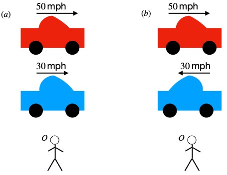
We’re all familiar with the concepts of Galilean relativity from everyday experience. It works like this: Imagine car A driving down the road at a speed of 30 mph rightward relative to Observer O on the side of the road. A car B is traveling along side car A at a speed of 50 mph rightward relative to Observer A (figure 1.1a). To the driver of car A, car B will appear to be moving at a speed of 50 mph – 20 mph = 20 mph past him.
If car A is driving at 30 mph rightward relative to Observer O and car B is driving leftward at 50 mph relative to O (figure 1.1b), then the driver of car A will see the speed of car B as -50 mph – 30 mph = -80 mph (i.e., 80 mph in a direction opposite him.
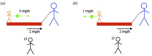
Furthermore, suppose a man is pulling a wagon at 2 mph on a sidewalk rightward with with respect to Observer O on the grass next to the sidewalk. A girl in the wagon throws a ball in the direction of motion at 5 mph (figure 1.2a). Observer O will see the ball traveling rightward at 2 mph + 5 mph = 7 mph.
Finally (figure 1.2b), consider the same setup as the last example, except this time, the girl throws the ball backward at 1 mph in her frame of reference (leftward according to O). Observer O will see the ball as traveling rightward at 1 mph.
This is all straightforward enough.
Now, fast-forward to the early twentieth century. By that time, Maxwell had developed a theory of electromagnetism that was regarded to be on the same solid footing as Newtonian mechanics and Newtonian gravity. At the turn of the century, a then unknown physicist working as a patent clerk in Switzerland, Albert Einstein, began to contemplate these issues. He recognized that problems arise when one attempts to apply Galilean relativity to electromagnetism.
Although Einstein didn’t mention the specific problem I’m about to describe in his original paper, figure 1.3 depicts the type of difficulty that Einstein identified.
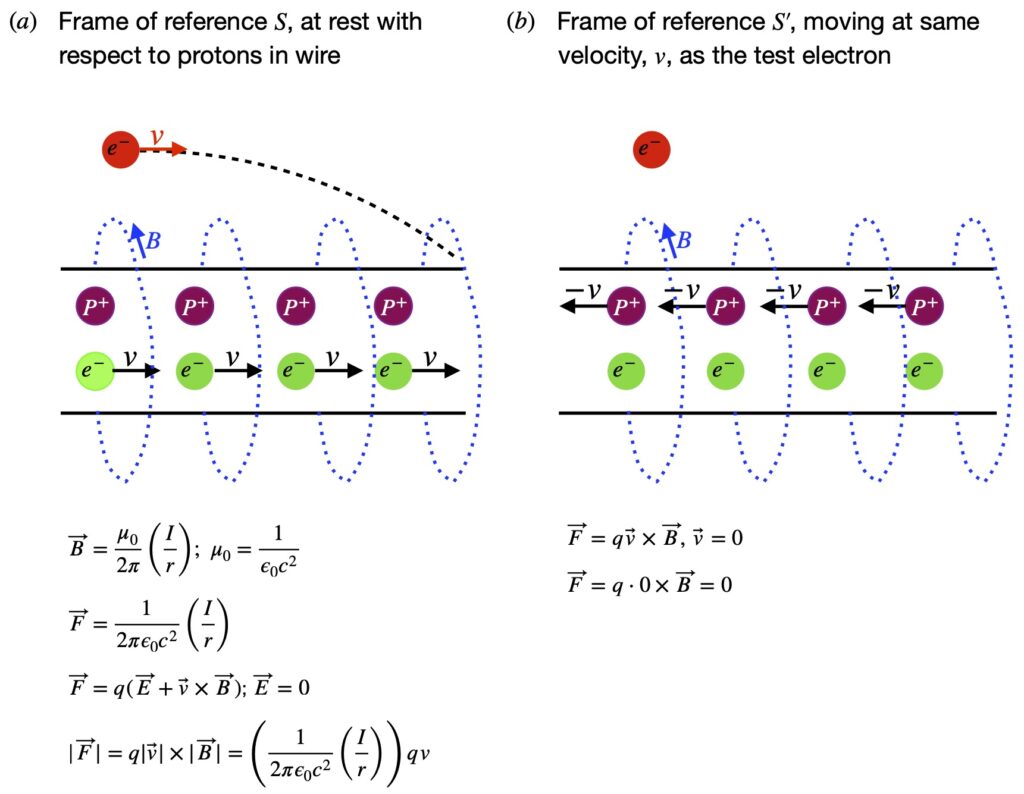
In figure 1.3a, we have reference frame S in which an observer (call her Observer S) sees a wire with fixed protons and mobile electrons, moving to the right at velocity,  , creating a current, which by convention, moves to the left (in the direction of positive charge). We fire in a test electron which our observer describes as moving to the right at velocity , the same velocity as the electrons in the wire.
In reference frame S´, our observer (call him Observer S´) takes the viewpoint of the test electron, which Observer S would say is traveling to the right at the same velocity as the mobile electrons in the wire. Observer S´ considers himself to be at rest and the electrons in the wire to be at rest. However, he sees the protons in the wire, which observer S considers stationary, as moving with velocity v to the left.
So what does the test electron experience from the viewpoint of Observer S. Well, the positive charges from protons in the wire are seen as balancing the electrical charge associated with the wire’s electrons. The wire, then, is seen as having zero net charge. Therefore, Observer S sees no electric field field. However, the electrons in the wire are moving. Such moving charge creates a magnetic field which gets weaker the further way from the wire one sits.
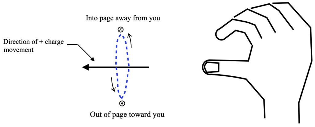
The direction of the magnetic field follows the right hand rule, depicted in figure 1.4b: point your thumb in the direction of movement of positive charge and curl your fingers. The direction in which your fingers point indicate the direction of the magnetic field. Figure 1.4a is a schematic of the direction of current flow and its associated magnetic field. It follows the convention that current flows in the direction of positive charge*.
*Only one “ring” of isotropic field strength is shown. In reality, there are an infinite number of isotropic rings of differing field strength, the strength of the field decreasing in proportion to the square of the ring’s distance away from the charge source.
In the figure 1.4a, the leftward-pointing arrow indicates the direction of movement of positive charge. In our example, negatively-charged electrons move to the right so, by convention, current flows to the left. The interrupted blue circle indicates the direction of the magnetic field. Again, per convention, the circle with the dot in the middle of it means that the magnetic field is coming out of the screen toward us while the circle with the x in it means that the magnetic field is moving into the screen, away from us.
I won’t derive the formulas from classical electromagnetism I use in this discussion; perhaps I’ll create a page showing these derivations in the future. Instead, for now, I’ll just state them and use them.
To start, it’s known that the magnitude of a magnetic field created by a moving charge is given as:
 where
where
 is the magnetic field vector created by the moving charge
 is the permeability of free space
 is the electrical current in the wire
 is the distance from the wire
We’ll change units to make subsequent math a little easier. Recognizing that
 where
where
 is the permittivity of free space
 is the speed of light
we write:

The force produced on a charged particle (in our case, the test electron) by an electric or magnetic field is given by the Lorentz force law:
 where
where
 is the force on the charged particle
 is the electric charge of the test particle
 is the electric field affecting the test particle
is the velocity of the test particle
 is the magnetic field effecting the test particle
 means take the cross product between to vectors, in this case and , in that order
Because the wire is electrically neutral, there is no electrical force on the test electron. Therefore, in our case, the Lorentz Force Law reduces to:

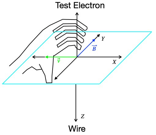
Let’s take a moment and talk about the cross product. The cross product is an operation which takes in two 3-dimensional vectors and results in a new vector. The magnitude of that new vector is obtained by multiplying the magnitudes of the individual vectors we’re taking the cross product of. Its direction can be obtained by a variety of methods. One is the right hand rule we’ve already discussed. Applied in the cross product operation, the fingers of the right hand are curled from the first vector in the cross product expression (in this case ) toward the second vector in the expression (in this case ). The direction in which the thumb is pointing is the direction of the resulting vector. As it applies to our magnetic force problem, the vector refers to the velocity of positive charge. In our case, a negatively charged electron is moving to the right. This is considered the same as positive charge moving to the left. The right hand in figure 1.5 is upside down with the palm facing us, indicating that, in our case of a magnetic field acting on a rightward moving test electron, the force on the test electron is downward, toward the wire.
The outcome of this interaction is that the test electron follows a parabolic path into the wire. The magnitude of the downward component of force on the test electron toward the wire is:

where the vertical lines on each side of a vector symbol indicates the magnitude of that vector.
Now let’s turn to the reference frame of Observer S´. He is traveling to the right with the test electron which, itself, is traveling with the same rightward velocity, , as the electron in the wire. Again, because the wire is electrically neutral, there is no electric field, so the Lorentz force equation again reduces to:

But in this case, Observer S´ sees the test electron as being at rest (i.e.,  ). Therefore, according to Observer S´, there is no force on the test electron. (Contrast this with the magnetic force on the test electron Observer S sees.) This troubled Einstein, who believed – as Galileo did – that the laws of physics should be the same in any frame of reference.
[Note that the above derivation is taken from Dr. Martin Smalley, https://www.youtube.com/watch?v=iUBiF2-1Tq4.]
Einstein also realized that manipulation of Maxwell’s equations predicts a constant value for the speed of light in a vacuum (approximately  meters per second). To see where this comes from, click .
 and current density
  . Thus,
 is the magnetic permeability constant and
  is the electric permittivity constant
![\[ \nabla \times (\nabla \times \vec{E}) = \nabla(\nabla \cdot \vec{E}) - \nabla^2\vec{E} \quad \text{eq 6}\]](https://www.samartigliere.com/wp-content/ql-cache/quicklatex.com-65b8903e77c08af4d158387c2b8c6e06_l3.png "Rendered by QuickLaTeX.com")
 , we have:

![\[ v^2 \frac{\partial^2 E}{\partial x^2} &= \frac{\partial^2 \vec{E}}{\partial t} \quad \text{eq 9}\]](https://www.samartigliere.com/wp-content/ql-cache/quicklatex.com-4a98aa72ed5d5bc666e340dded58e36b_l3.png "Rendered by QuickLaTeX.com")


Albert Michelson (the same Michelson who would later say that there was nothing left in physics to discover) subsequently confirmed this prediction by experiment. Furthermore, in 1887 Michelson and Edward Morley, in attempting to prove the existence of a medium through which light traveled called the ether, proved just the opposite: that the speed of light seemed to be the same no matter in what direction it was measured. (For details, click here.)
Given these facts, Einstein postulated that the speed of light was the same in all reference frames.
But there was a problem. If one applies Galilean relativity to objects traveling near the speed of light, things didn’t work out so well. To see this, suppose Observer S is sitting still in outer space, in a frame of reference that we’ll call S. Observer S watches Observer S´, traveling from his left to his right (the + direction in Observer ‘S‘s frame of reference), in a rocket ship, at a constant velocity of 0.5 times the speed of light (= 0.5c, where c = the speed of light = meters per second). Simultaneously, a light beam moves past Observer S, right to left. What we want to know is, at what velocity does Observer S´ say the beam of light is traveling.
According to Galilean relativity,Observer S´ should measure the speed of the light beam as -1.5c (i.e., -c – 0.5c = -1.5c). But this contradicts the idea that the speed of light is constant (equal to c) in all inertial frames. Einstein realized that either Maxwell’s theory was wrong (the speed of light is not constant) or Galilean relativity was wrong. Einstein banked on the latter. The result was his 1905 landmark paper “On the Electrodynamics of Moving Bodies” which outlined his theory of special relativity. You can find a copy of it here:
https://www.fourmilab.ch/etexts/einstein/specrel/specrel.pdf
In it, he begins with two postulates:
- The laws of physics are the same in all inertial frames of reference (i.e., frames of reference where objects are moving at constant velocity)
- The speed of light is constant in all inertial frames of reference
Einstein recognized that, if these postulates were true, then Galilean relativity had to be revised. Namely, if time moved more slowly and units of length became shorter in frames of reference moving with respect to an observer, especially as the velocity approached the speed of light, then the invariant nature of the speed of light would be preserved. Such behavior of space and time would also solve the discordance between non-relativistic physics and electromagnetism. To see the counterintuitive specifics of Einstein’s theory, read on.
II. Loss of Simultaneity
Imagine an observer, Observer B, on the platform of a train station (figure 2.1). A train goes by Observer B traveling 30 mph to her right. In the middle of the train is an observer, Observer A. Observer A has two machines that fires tennis balls toward the front and back of the train at 50 mph.
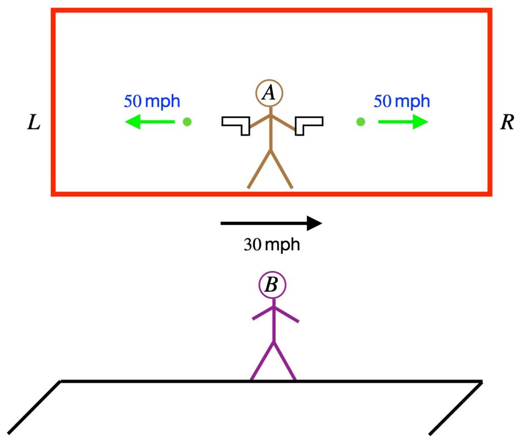
Like any observer in their own frame of reference, Observer A thinks he’s at rest. He see the tennis balls hit the left and right sides of the train simultaneously.
What about Observer B? In her frame of reference, the gun firing the tennis ball toward L is moving at 30 mph to the right. The ball is fired at 50 mph to the left so the net velocity of the ball from Observer B’s viewpoint is 20 mph to the left. However, the left wall of the train is moving at the ball at 30 mph so the “gap” between the ball and the wall are closing at 20 mph – (-30 mph) = 50 mph. At the same time, the rightward traveling ball’s velocity, according to Observer B, is 30 mph due to the motion of the train + 50 mph due to the velocity the machine =. 50 mph. However, the righthand wall of the train is receding from the ball at 30 mph. Therefore, the gap between the rightward traveling ball and receding righthand wall of the train is closing at 80 mph – 30 mph = 50 mph, same as for the leftward traveling ball and rightward traveling left wall of the train. Thus, ignoring an inconsequential (at this velocity) correction due to special relativity, Observer B sees the balls hit the right and left walls of the train at the same time.
Now consider what happens if we measure the time that light beams shined rightward and leftward from the middle of a similar train hits the right and left walls (figure 2.2). Again, there are 2 observers, Observer A on the train and Observer B on the train station platform, and again, the train is moving rightward with respect to Observer B at velocity  . And per Einstein’s second postulate of special relativity, the speed of light,
  , is the same in all inertial frames of reference.
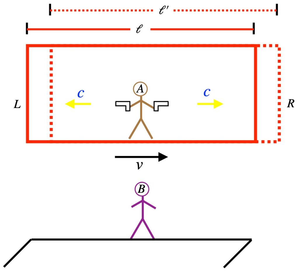
What will Observer A see? Well, Observer A sees himself, the light guns the light beams and the walls as stationary. If the length of the train is  , then the time it takes for the leftward-directed light beam to hit the lefthand wall is

 is the time it takes for the leftward light beam to hit the left wall
is the length of the train
is the speed of light
Likewise, the time it takes for the rightward-directed light beam to hit the righthand wall is also

 is the time it takes for the rightward beam to hit the right wall.
That is, the light beams hit the left and right walls of the train simultaneously. Now what does Observer B observe?
First off, unlike the tennis balls, in which different observers see different velocities depending on the frame of reference, the speed of light is constant in all inertial frames. Using this fact, we can calculate the time it takes for the light beams to hit the left and right hand walls in Observer B’s frame. First, the left side.
We know that the rate at which the gap between the rightward-traveling lefthand wall and light beam closes is  . Note that I’m not saying that the light beam is traveling at
  . The light, as always, travels at . What I’m saying is the “gap” between the left wall and the light beam is decreasing at . Similarly, the gap between the rightward traveling light beam and receding righthand wall is closing at a rate of
  . Thus,

Even though and  may be different due to the relativistic effect of length contraction (discussed below), the effect is the same everywhere. Therefore, it has no effect on the relative values of and . The values of and are still different. Therefore, unlike the arrival of light at the left and right walls of the train in Observer A’s frame of reference – which is simultaneous – these events, in Observer B’s frame of reference, are NOT simultaneous. And if the train were moving in the opposite direction, Observer B would see the light beam hit the righthand wall AFTER it hits the lefthand wall.
In short, the relative timing of events depends on the frame of reference in which it is being observed.
This discussion is patterned after David Morin at https://scholar.harvard.edu/files/david-morin/files/relativity_chap_1.pdf
III. Time Dilation
In special relativity, to Observer A, an object (Object B) moving with constant velocity relative to Observer A will perceive a clock moving with Object B as ticking slower than a clock they are holding. This is called time dilatation.
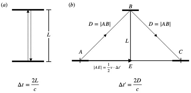
Figure 3.1a shows a clock of sorts in which a beam of light is sent straight upward, hits a mirror  units away, then reflects back, striking a detector at the site from which it originated. The total distance that the light beam travels during this trip is
  . Observer A standing at rest relative to the light source measures the elapsed time for this round trip as
  . The speed of the light beam is the speed of light, . Now
  . Therefore,
  .
.
Applying this to figure 3.1a, we can see that

In figure 3.1b, Observer A remains at point A. The light source at A emits a light beam toward B then starts moving to the right at velocity . A mirror sitting at point B, a distance above the plane at which the light source was emitted (and halfway between points A and C), reflects the beam. The moving detector (which is adjacent to the light source) detects the light beam that it previously sent, at point C. Observer A measures the time it takes the detector plate to move from A to C as  . The distance the detector travels from A to C is given by
  . The light travels a distance
  from A to the mirror at B then another distance from the mirror to the detector at C. The total distance for the trip is
  . Thus, the time that Observer A measures the time the light beam takes on its journey from A to B to C as

Our ultimate task is to relate  and
and  . To do this, we note that lines connecting A, B and E create a right triangle. We see from figure 1b that

From the Pythagorean theorem


But
Therefore
 Square both sides
 Subtract
  from both sides
 Factor out
  from the left side
 Divide both sides by
 Take the square root of both sides

But we know from figure 1a that  , so
, so

In the literature, the term that multiplies is referred to as gamma:

Let’s see how this equation can be applied. Let’s examine a dramatic example. Suppose the moving detector is traveling at 75% the speed of light (i.e.,  ). Observer A’s clock ticks 1 second (i.e.,
  ). Plugging in these values, we get:

This means that, in the time Observer A’s clock ticks 1 second, Observer A perceives a clock on the moving detector as having ticked 2 seconds. That is, Observer A thinks the clock on the moving detector is ticking slower than their clock (i.e., time has “dilated”).
Note that the time measured in the moving frame of reference (in our case here referred to as ) is often referred to as coordinate time. On the other hand, the time measured by an observer in the same frame of reference as the clock that’s measuring it is called the proper time. In this case, it’s what we’re calling . Proper time, in special relativity, is an invariant quantity. That is, observers in all frames of reference will measure this same quantity. Or stated in more formal terms, proper time is a Lorentz scalar. A scalar is an entity that’s just a number. It doesn’t change no matter what coordinate system one is using. A Lorentz scalar is an entity that doesn’t change under a coordinate transformation called a Lorentz transformation. More about this later.
The discussion presented in this section as well as the basic plan for figure 3.1 were taken from Wikepidia https://en.wikipedia.org/wiki/Time_dilation.
IV. Length Contraction
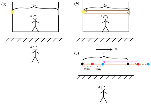
In special relativity, an object in a frame of reference that is moving relative to an observer, Observer A, will be measured by Observer A as being shorter than Observer A measures the object in his or her own frame of reference. This is illustrated in figure 4.1.
In figure 4.1a, we have two observers: Observer B who is inside a train and Observer A who is outside the train. Both are at rest. The length of the train measures  in B’s frame of reference. Because this length is being measured in the frame of reference in which the length exists, is referred to as a proper length. On the left-hand side of the train is a light source (yellow circle) which doubles as a photon receptor. On the right wall of the train is a mirror (vertically-oriented gray band). Since Observers B is not moving relative to Observer A, A also measures the length of the train as .
In figure 4.1b, Observer B clicks on the light source which sends a light ray from the source to the mirror. The mirror reflects the light back to the source where it is detected. Observer B measures the time it takes for the light beam to complete this round trip as
![\[\Delta t_0 =\displaystyle \frac{L_0}{c} \quad \text{eq (4.1)} \]](https://www.samartigliere.com/wp-content/ql-cache/quicklatex.com-b2286b5514c7a8b5a8e96606c37d1212_l3.png "Rendered by QuickLaTeX.com")
Observer A (not shown in figure 4.1b) is still at rest with respect to B and thus measures the same time for the light’s round trip.
What happens if the train is set in motion, to the right, at velocity ? What does Observer A see? This is depicted in figure 4.1c. In this figure, to avoid clutter, the train is not shown. Only the light source and the mirror are shown (at various times/positions).
The light , whose course is depicted as the rightward brown arrow, will eventually hit the mirror . In her stationary frame of reference, Observer A measures the time at which this occurs as  . However, to hit the mirror, the light must travel the length of the train, plus the distance the train has traveled over which is given
  . The point at which the light hits the mirror is at the right-hand red dot. Observer A measures the time that the light travels before hitting the mirror as:
![\[ \Delta t_1 = \frac{\displaystyle L + v \Delta t_1}{\displaystyle c} \quad \text{eq (4.2)} \]](https://www.samartigliere.com/wp-content/ql-cache/quicklatex.com-9a885e4291d104879993e6a7a856676a_l3.png "Rendered by QuickLaTeX.com")
Rearranging, we find:

Note that we’re considering the possibility that the length of the train measured by A with the train moving () may not be the same as the length of the train measured by Observer B or Observer A with the train at rest ().
At any rate, the light is reflected and eventually detected at the left-hand side of the train, at the left-hand blue dot. Observer A measures the time it takes for the light to get from the mirror to the detector as  . Notice that during this time, in A’s frame of reference, , the left-hand side of the train where the detector is has moved a distance
  to the right. Therefore, per Observer A, the distance the light travels from the mirror to the detector is
![\[ \Delta t_2 = \frac{\displaystyle L - v \cdot \Delta t_2}{\displaystyle c} \quad \text{eq (4.4)} \]](https://www.samartigliere.com/wp-content/ql-cache/quicklatex.com-9287dce67babd3dfb65093c923100228_l3.png "Rendered by QuickLaTeX.com")
Manipulating this equation in a manner similar to what we did before, we ultimately wind up with:
![\[ \Delta t_2 &= \displaystyle \frac{\displaystyle L}{\displaystyle c+v} \quad \text{eq (4.5)} \]](https://www.samartigliere.com/wp-content/ql-cache/quicklatex.com-d5f36a40c4d61952fb56c5c143fe339c_l3.png "Rendered by QuickLaTeX.com")
Observer A measures the total time the light takes to go from the source to the mirror and back to the source as

We can relate  and using the equations we derived in the last section on time dilatation:
![\[ \Delta \, t^{\prime} = \frac{\displaystyle \Delta \, t}{\displaystyle \sqrt{1 - \displaystyle \frac{\displaystyle v^2}{\displaystyle c^2} }} \quad \text{eq (3.6)} \]](https://www.samartigliere.com/wp-content/ql-cache/quicklatex.com-efe441d8e82e3a6e7b48840f571239b0_l3.png "Rendered by QuickLaTeX.com")
However, we need to be careful about which time expressions we substitute where. In our current case, proper time – the time measured in train’s frame of reference i.e., that measured by Observer B (and Observer A with the train at rest) – is given as . This correlates with in the equation above. On the other hand, so-called coordinate time – the time measured by Observer A for the moving train – is referred to as in our current discussion. This correlates with in the time dilatation equation.
Given these considerations, then, we can write:
![\[ \Delta \, t = \frac{\displaystyle \Delta \, t_0}{\displaystyle \sqrt{1 - \displaystyle \frac{\displaystyle v^2}{\displaystyle c^2} }} \quad \text{eq (4.7)} \]](https://www.samartigliere.com/wp-content/ql-cache/quicklatex.com-16330969ac16b1694213e3352166058d_l3.png "Rendered by QuickLaTeX.com")
Plugging in our values for and  , then doing some algebra, we obtain:

Since  is < 1, this equation indicates that , the length of the train measured by A in the moving reference frame, is smaller than , the length of the train in the rest frame – the proper length. That is, length contraction has occurred.
The arguments put forth in this section as well as figure 4.1 where patterned after the Faculty of Khan video at https://www.youtube.com/watch?v=DJKDF86Ebnw.
V. Spacetime Diagrams
A useful tool in the study of special relativity is the spacetime diagram. This will prove particularly useful in elucidating the relationship between coordinates in different frames of reference – the so-called Lorentz transformations.
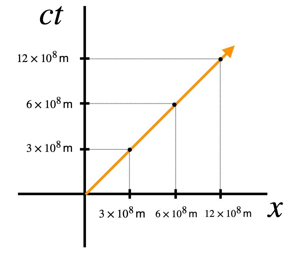
One of the prime tenants of special relativity is that space and time are both parts of one continuum: spacetime. When we plot graphs of position versus time in regular classical mechanics, we think of three spatial dimensions, which we’ll call x, y and z, and a separate time dimension. In special relativity, on the other hand, we consider time on the same footing as spatial dimensions. Indeed, what we plot in a so-called spacetime diagram as time is actually the speed of light, c, multiplied by time, t, to give us ct, the “time” dimension in spacetime. When we do this, the units measured on the “time” axis now has units of length. So, for example, if we’re working in units of light-seconds, then 3.0 x 10⁸ meters/second x 1 second = 3.0 x 10⁸ meters. The distance that light travels in 1 second along the x direction is 3.0 x 10⁸ meters. Thus, 1 unit in the ct dimension is the same as 1 unit in the x direction. We plot light rays on these spacetime diagrams, then, as lines at 45° angles, as shown in figure 5.1.
Now let’s consider Observer S floating in space. Like any observer in their own frame of reference, Observer S thinks he’s at rest. Observer S´ is piloting a rocket, in a train of rockets, all traveling toward Observer S at 0.5 times the speed of light (0.5c), all 3 x 10⁸ m/s (meters/second). Like all observers in their own frame of reference, because the rockets are all moving at the same speed, Observer S´ considers herself and the rocket in front of her as stationary. She experiences “movement in time” but no movement in the x direction.
1 second (or 3 x 10⁸ m since we’re working in spacetime units) before she passes Observer S, Observer S´ emits a light ray in the positive x direction. In figure 5.2a, this is depicted by the orange line, a line that makes an angle of 45° with the ct´-axis (and -45° with the x´-axis) since we’re working in units in which 1 unit on the ct´-axis equals 1 unit on the x´-axis.
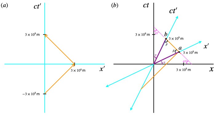
After 1 second, Observer S´, in her own frame of reference, has “moved forward in time” to ct´ = 0, the time at which she and Observer S, pass each other. (Note that, at time ct´ = 0, Observer S sees Observer S´ in her rocket pass him traveling to the right while Observer S´ sees Observer S passing her to the left at 0.5c.
Also at time ct´ = 0, Observer S´s light ray reflects off a mirror on the back of the rocket in front of her (point a) and reaches her again at ct´ = 1 second (point b).
Figure 5.2b shows the axes of Observer S’s frame of reference in black with the axes of Observer S´ s frame of reference superimposed in cyan. The orange line oriented at 45° represents the light ray she emits. Observer S’s ct´ axis is angled to the right, indicating a component of velocity in the positive x direction relative to Observer S. The angle of Observer S’s ct´ axis relative to Observer S’s ct axis is given by tan 𝛼 = v/c. This makes sense since v represents the x-component of Observer S’s ct´ axis and c its ct component.
But what about the Observer S’s x´ axis? What angle does it make with Observer S’s x-axis? Well, we know from figure 2a that the point where the light ray hits the mirror, point a, is the point on Observer S’s x´ axis x´ = 3.0 x 10⁸ m. In this spacetime diagram, it then makes an angle of 90° with the x´ axis and eventually arrives back at Observer S´ at ct´ = 3.0 x 10⁸ m, at point b. So we’ve now defined 2 points on the x´ axis: x´ = 0, ct´ = 0 and x´ = 3.0 x 10⁸ m, ct´ =0. Two points are all we need to draw a line, in this case the x´-axis. Now for the angle it makes with the x-axis.
Referring to figure 5.2b, we know that extensions of the light path from the x´-axis to the ct´-axis (magenta dotted lines in the diagram) make 45° angles with the x– and ct axes, respectively. Distances from the origin to point a and point b (depicted in purple in the diagram) form the sides of an isosceles triangle. From geometry, we know, then, that the angles labeled ß are equal. The angles complementary to angle ß around points a and b equal 180 – ß. The triangles from the origin to point a to the x´-axis and from the origin to point b to the ct´-axis have 2 angles that are the same: 45° and 180° – ß. Since the angles of a triangle (at least in flat space) must equal 180°, the angles 𝛼 between the ct´- and ct-axes and the x´- and x-axes must be equal. The primed axes are also always symmetric about the 45°-angled path of a light ray. The closer the speed of the moving frame of reference those axes represent get to the speed of light, the closer the axes get to the 45° light ray path. This variation in axis configuration in the moving frame reflects the effects of time dilation and length contraction needed to keep the speed of light constant in all reference frames.
VI. Lorentz Transformation
With knowledge of spacetime diagrams in hand, let’s make such a diagram to help us derive the formulas for the Lorentz transformations For simplicity, we’ll consider only one spatial dimension in the following derivation because the same arguments we apply to this one spatial dimension can easily be applied to each of the other two spatial dimensions.
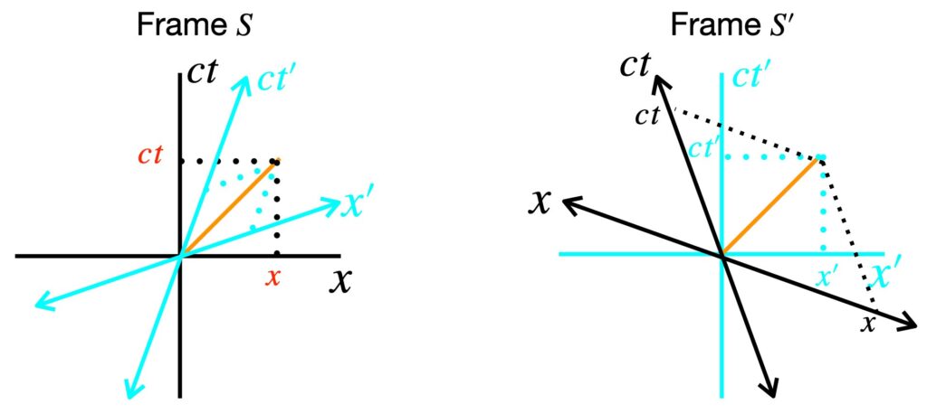
The diagram on the left represents the frame of rest of an observer, Observer S, floating in space. Like any observer in their own frame of reference, Observer S believes she is at rest. The black coordinate axes in the diagram on the left represent the coordinates that correspond to Observer S.
Observer S sees a rocket go by at velocity v relative to her. Of course, the pilot of the rocket, Observer S´, thinks he’s at rest and sees Observer S moving to the left with velocity v. His coordinates are shown in cyan and are labeled as ct´ and x´ in the diagram on the right.
Superimposed on the coordinates of Observer S in frame S, in cyan, are the coordinates of Observer S´. Similarly, superimposed on the coordinates of S´, in black, in frame S´, are the coordinates of Observer S. Notice that they point in a direction opposite to the coordinates of Observer S´ in frames S. This is because Observer S´ sees Observer S moving to the left.
What we want to do, in this section, is to find expressions that relate the x and ct coordinates of Observer S to the x and ct coordinates of Observer S´(which we’ll refer to as x´ and ct´). These expressions are called Lorentz transformations after Dutch physicist Hendrick Lorentz, who discovered them. There are a number of ways to derive such expressions. The derivation that follows is taken from Khan Academy, https://www.khanacademy.org/science/physics/special-relativity/lorentz-transformation/v/lorentz-transformation-derivation-part-1
Let’s begin by trying to come up with equations for x´ and x. A good start would be to use Galilean transformations  for Observer S and
  for S´ (
 for the S´ frame because Observer S´ sees Observer S moving to the left). But we know that time dilation and length contraction must be taken into account. Therefore, perhaps, we should add a scaling factor which we’ll call
  . We know that the lengths of units on coordinate axes in a given frame of reference are equal everywhere (although the length of those units will vary from inertial frame to inertial frame). Due to this homogeneity, we can make the assumption that our scaling factor will be linear. And because of the symmetry of frames S and S´, we will make the educated guess that the same scaling factor applies to expressions for both the x and x´. When we do, we get:
![\[x^{\prime}=\gamma(x-vt)\quad \quad \text{eq (6.1)}\]](https://www.samartigliere.com/wp-content/ql-cache/quicklatex.com-df0722b754ee04cc7fd438490bef39e9_l3.png "Rendered by QuickLaTeX.com")
and
![\[x = \gamma(x^{\prime} + vt^{\prime})\quad \quad \text{eq (6.2)}\]](https://www.samartigliere.com/wp-content/ql-cache/quicklatex.com-a17f1ea5d81e995eff609c959145866e_l3.png "Rendered by QuickLaTeX.com")
Multiply eq (6.1) by x. We get:

From the diagram, we know that the equation for the orange line representing the light ray in frame S is  and frame S´ is
  . Substituting these values for x and x´ into eq (6.3) gives us:

Now that we’ve got an expression for our scaling factor , we can plug it into equations (6.1) and (6.2) to obtain the Lorentz transformations for x and x´:
![\[x^{\prime} =\frac{1}{\sqrt{1-\frac{v^2}{c^2}}} (x + vt)\quad \quad \text{eq (6.5)}\]](https://www.samartigliere.com/wp-content/ql-cache/quicklatex.com-8459cb3f5d6680e7a9f35766b94d0936_l3.png "Rendered by QuickLaTeX.com")
and
![\[x = \frac{1}{\sqrt{1-\frac{v^2}{c^2}}}(x^{\prime} + vt^{\prime})\quad \quad \text{eq (6.6)}\]](https://www.samartigliere.com/wp-content/ql-cache/quicklatex.com-b8f4008770e2b56280f633f9b8bb87f9_l3.png "Rendered by QuickLaTeX.com")
What we need to do next is find the Lorentz transformations for t and t´. To do this, we begin with equations (6.5) and (6.6) then perform some algebraic manipulation. Let’s start by finding the Lorentz transformation for t´:

We can modify this equation further to put it into the form that is most recognized:
![\begin{align*} t^{\prime} &= \gamma(\frac{x}{\gamma^2 v} - \frac{x}{v} + t) \quad \quad \text{expand}\\ &= \frac{x}{\gamma v} - \frac{\gamma x}{v} +\frac{\cancel{v} t \gamma}{\cancel{v}}\\ &= \frac{x}{\gamma v} - \frac{\gamma x}{v} + \gamma t \quad \quad \text{factor out } \gamma\\ &= \gamma\left[ \left( \frac{x}{\gamma^2 v} - \frac{x}{v} \right) + t \right] \quad \quad \text{factor out } x \text{ from } ()\\ &= \gamma \left[ x\left( \frac{1}{\gamma^2 v} - \frac{1}{v} \right) + t \right] \quad \quad \text{multiply } 1 \times \frac{1}{v}\\ &= \gamma \left[ x\left( \frac{1}{\gamma^2 v} - \frac{\gamma^2}{\gamma^2} \cdot \frac{1}{v} \right) + t \right] \quad \quad \text{expand and simplify}\\ &= \gamma \left[ x\left( \frac{1-\gamma^2}{\gamma^2 v} \right) + t \right] \quad \quad \text{eq (6.8)} \end{align*}](https://www.samartigliere.com/wp-content/ql-cache/quicklatex.com-0daa948ff788f276435ac71c8b5984be_l3.png "Rendered by QuickLaTeX.com")
From here, we note that
![\[ \gamma = \frac{1}{\sqrt{1-\frac{v^2}{c^2}}} \,\, \Rightarrow \,\, \gamma^2 = \frac{1}{1-\frac{v^2}{c^2}} \cdot \frac{c^2}{c^2} = \frac{c^2}{c^2-v^2} \quad \quad \text{eq (6.9)} \]](https://www.samartigliere.com/wp-content/ql-cache/quicklatex.com-cc07cd110eba1079312be86c59ebb531_l3.png "Rendered by QuickLaTeX.com")
We make use of this to modify the expression  in eq (6.8):
![\begin{align*} t^{\prime} &= \gamma\left[ x \left( \displaystyle \frac{\displaystyle \frac{c^2-v^2}{c^2-v^2} - \displaystyle \frac{c^2}{c^2-v^2}}{\displaystyle \frac{c^2 v}{c^2-v^2}} \right) + t \right]\\ \\ &= \gamma \left[ x \left( \displaystyle \frac{\displaystyle \frac{-v^2}{c^2-v^2}}{\displaystyle \frac{c^2 v}{c^2-v^2}} \right) + t \right]\\ \\ &= \gamma \left[ x \left( \displaystyle \frac{-v^2}{\cancel{c^2-v^2}} \cdot \displaystyle \frac{\cancel{c^2-v^2}}{c^2 v} \right) + t \right]\\ \\ &= \gamma \left[ x \left( \displaystyle \frac{-v^2}{c^2 v} \right) + t \right]\\ \\ &= \gamma \left( t - \displaystyle \frac{vx}{c^2} \right) \end{align*}](https://www.samartigliere.com/wp-content/ql-cache/quicklatex.com-6505071442f1cfd5252f8fc1a5ea11d8_l3.png "Rendered by QuickLaTeX.com")
So now we have an expression for the Lorentz transform for  :
:
![\[ t^{\prime} = \gamma \left( t - \displaystyle \frac{vx}{c^2} \right) \quad \quad \text{eq (6.10)}\]](https://www.samartigliere.com/wp-content/ql-cache/quicklatex.com-580b6b3b3132657824c2ae27aee354c4_l3.png "Rendered by QuickLaTeX.com")
We can derive an expression for  as well:
![\[ t = \gamma \left( t ^{\prime}+ \displaystyle \frac{vx^{\prime}}{c^2} \right) \quad \quad \text{eq (6.11)}\]](https://www.samartigliere.com/wp-content/ql-cache/quicklatex.com-967b0f28e4f0ea7769b768f5937ffb86_l3.png "Rendered by QuickLaTeX.com")
We could do this in a manner similar to the way we derived the expression for except we start with the equation  . To see the proof, click .

![\begin{align*} t &= \gamma(\frac{-x^{\prime}}{\gamma^2 v} + \frac{x^{\prime}}{v} + t^{\prime}) \quad \quad \text{expand}\\ &= \frac{-x^{\prime}}{\gamma v} + \frac{\gamma x^{\prime}}{v} +\frac{\cancel{v} t^{\prime} \gamma}{\cancel{v}}\\ &= \frac{-x^{\prime}}{\gamma v} + \frac{\gamma x^{\prime}}{v} + \gamma t^{\prime} \quad \quad \text{factor out } \gamma\\ &= \gamma\left[ \left( \frac{-x^{\prime}}{\gamma^2 v} + \frac{x^{\prime}}{v} \right) + t^{\prime} \right] \quad \quad \text{factor out } x^{\prime} \text{ from } ()\\ &= \gamma \left[ x^{\prime}\left( \frac{-1}{\gamma^2 v} + \frac{1}{v} \right) + t^{\prime} \right] \quad \quad \text{multiply } 1 \times \frac{1}{v}\\ &= \gamma \left[ x^{\prime} \left( \frac{-1}{\gamma^2 v} + \frac{\gamma^2}{\gamma^2} \cdot \frac{1}{v} \right) + t^{\prime} \right] \quad \quad \text{expand and simplify}\\ &= \gamma \left[ x^{\prime} \left( \frac{-1 + \gamma^2}{\gamma^2 v} \right) + t^{\prime} \right] \text{multiply } \frac{-1 + \gamma^2}{\gamma^2 v} \text{by } \frac{-1}{-1}\\ &= \gamma \left[ x^{\prime} \left( \frac{1 - \gamma^2}{-\gamma^2 v} \right) + t^{\prime} \right] \quad \quad \text{eq (6.8a)}\\ \end{align*}](https://www.samartigliere.com/wp-content/ql-cache/quicklatex.com-f2a343e0f62dcdb0eb8d930f5d8ad188_l3.png "Rendered by QuickLaTeX.com")
![\[ \gamma = \frac{1}{\sqrt{1-\frac{v^2}{c^2}}} \,\, \Rightarrow \,\, \gamma^2 = \frac{1}{1-\frac{v^2}{c^2}} \cdot \frac{c^2}{c^2} = \frac{c^2}{c^2-v^2} \]](https://www.samartigliere.com/wp-content/ql-cache/quicklatex.com-db8a7310058ed2ed9e522c981caccd2c_l3.png "Rendered by QuickLaTeX.com")
 in eq (6.8a):
![\begin{align*} t &= \gamma\left[ x^{\prime} \left( \displaystyle \frac{\displaystyle \frac{c^2-v^2}{c^2-v^2} - \displaystyle \frac{c^2}{c^2-v^2}}{\displaystyle \frac{-c^2 v}{c^2-v^2}} \right) + t^{\prime} \right]\\ \\ &= \gamma \left[ x^{\prime} \left( \displaystyle \frac{\displaystyle \frac{-v^2}{c^2-v^2}}{\displaystyle \frac{-c^2 v}{c^2-v^2}} \right) + t^{\prime} \right]\\ \\ &= \gamma \left[ x^{\prime} \left( \displaystyle \frac{-v^2}{\cancel{c^2-v^2}} \cdot \displaystyle \frac{\cancel{c^2-v^2}}{-c^2 v} \right) + t^{\prime} \right]\\ \\ &= \gamma \left[ x^{\prime} \left( \displaystyle \frac{v^2}{c^2 v} \right) + t^{\prime} \right]\\ \\ &= \gamma \left( t^{\prime} + \displaystyle \frac{vx^{\prime}}{c^2} \right) \end{align*}](https://www.samartigliere.com/wp-content/ql-cache/quicklatex.com-41ecda0b015ef869f9222fc9a14b8833_l3.png "Rendered by QuickLaTeX.com")
Here is a summary of the Lorentz transform equations:
![\[x^{\prime} =\frac{1}{\sqrt{1-\frac{v^2}{c^2}}} (x - vt)\quad \quad \,\text{eq (6.5)}\]](https://www.samartigliere.com/wp-content/ql-cache/quicklatex.com-264d8b044d022d7ccbbf43ca7a2f567e_l3.png "Rendered by QuickLaTeX.com")
![\[t^{\prime} = \gamma \left( t - \displaystyle \frac{vx}{c^2} \right) \quad \quad \quad \quad \,\,\,\,\text{eq (6.10)}\]](https://www.samartigliere.com/wp-content/ql-cache/quicklatex.com-b2afd62bd10a27d9a8d77ccf0afe1e7f_l3.png "Rendered by QuickLaTeX.com")
![\[t = \gamma \left( t ^{\prime}+ \displaystyle \frac{vx^{\prime}}{c^2} \right) \quad \quad \quad \quad \,\text{eq (6.11)}\]](https://www.samartigliere.com/wp-content/ql-cache/quicklatex.com-bb867d670190bc0f0afa70193c8ec853_l3.png "Rendered by QuickLaTeX.com")
A useful way to work with these equations is to put them into matrix form using the so-called Lorentz transformation matrix. Here’s what it looks like:
![\[ \begin{pmatrix} t^{\prime}\\ x^{\prime}\\ y^{\prime}\\ z^{\prime} \end{pmatrix} = \begin{pmatrix} \gamma & -\gamma v/c^2 & 0 & 0\\ -\gamma v & \gamma & 0 & 0\\ 0 & 0 & 1 & 0\\ 0 & 0 & 0 & 1 \end{pmatrix} \begin{pmatrix} t\\ x\\ y\\ z \end{pmatrix} \quad \quad \text{eq (6.12)}\]](https://www.samartigliere.com/wp-content/ql-cache/quicklatex.com-458a061d8248213efeb3658cb2ad0e01_l3.png "Rendered by QuickLaTeX.com")
For readers that need some help with matrix multiplication, click .
 ,
,  and
and  values, respectively, of the frame S´ column vector, as shown in figures (b), (c) and (d), respectively.
Eq (6.12) is the matrix equation that transforms coordinates when there is relative motion in the x-direction. Similar matrices can be constructed to transform vectors when there is relative motion in the y- and z-directions. For the y-direction, we have:
![\[B_y =\begin{pmatrix}\gamma & 0 & -\gamma v/c^2 & 0\\0 & 1 & 0 & 0\\-\gamma v & 0 & \gamma & 0\\0 & 0 & 0 & 1\end{pmatrix}\quad \text{eq (6.13)}\]](https://www.samartigliere.com/wp-content/ql-cache/quicklatex.com-e353842f935e7002fb6cd6342631baff_l3.png "Rendered by QuickLaTeX.com")
For relative motion in the z-direction, we use:
![\[B_z =\begin{pmatrix}\gamma & 0 & 0 & -\gamma v/c^2\\0 & 0 & 0 & 0\\0 & 0 & 1 & 0\\-\gamma v & 0 & 0 & \gamma\end{pmatrix}\quad \text{eq (6.14)}\]](https://www.samartigliere.com/wp-content/ql-cache/quicklatex.com-06c21c41455ba58eebc0a8bf554a9d6f_l3.png "Rendered by QuickLaTeX.com")
In eq (6.13) and eq (6.14),  stands for boost in the direction of
  . A boost simply represents transformation to a frame of reference with motion in the direction relative to some other frame of reference. So if coordinate system
  is moving in the y-direction relative to coordinate system
  , then that’s referred to as a boost in the y-direction.
Spatial rotations can also be represented by matrices in special relativity. Matrices representing pure spatial rotations include:
Around the x-axis:
![\[R_{\theta_z}=\begin{pmatrix} 1 & 0 & 0 & 0 \\ 0 & 1 & 0 & 0 \\ 0 & 0 & \cos \theta & -\sin \theta \\ 0 & 0 & \sin \theta & \cos \theta \end{pmatrix} \quad \text{eq (6.15)} \]](https://www.samartigliere.com/wp-content/ql-cache/quicklatex.com-98bd259275ecb387cc2f6f5b2d0ec146_l3.png "Rendered by QuickLaTeX.com")
Around the y-axis:
![\[R_{\theta_y}=\begin{pmatrix} 1 & 0 & 0 & 0 \\ 0 & \cos \theta & 0 & -\sin \theta \\ 0 & 0 & 0 & 0 \\ 0 & 0 & \sin \theta & \cos \theta \quad \text{eq (6.16)} \end{pmatrix}\]](https://www.samartigliere.com/wp-content/ql-cache/quicklatex.com-b5ce45050b6587f85f7bc60fe669e126_l3.png "Rendered by QuickLaTeX.com")
Around the z-axis:
![\[ R_{\theta_z}=\begin{pmatrix} 1 & 0 & 0 & 0 \\ 0 & \cos \theta & -\sin \theta & 0 \\ 0 & \sin \theta & \cos \theta & 0 \\ 0 & 0 & 0 & 0 \end{pmatrix} \quad \text{eq (6.17)}\]](https://www.samartigliere.com/wp-content/ql-cache/quicklatex.com-3f2adc722c2e35bf4ab99532cd32a66c_l3.png "Rendered by QuickLaTeX.com")
We can combine boosts, , and rotations,  by performing matrix multiplication. For example, a boost in the x direction followed by a rotation around the z-axis would be accomplished mathematically by:
![\[ \vec{x}\,^{\prime} = R_{\theta_z} B_x\, \vec{x}\]](https://www.samartigliere.com/wp-content/ql-cache/quicklatex.com-80272639ca603652970712aab65825ae_l3.png "Rendered by QuickLaTeX.com")
or

Another well-known example of this is the so-called Thomas-Wigner rotation. This refers to the fact that 2 boosts can be shown to be equivalent to one boost and one rotation. Intuition as to why this is so can be gleaned from figure 6.2.
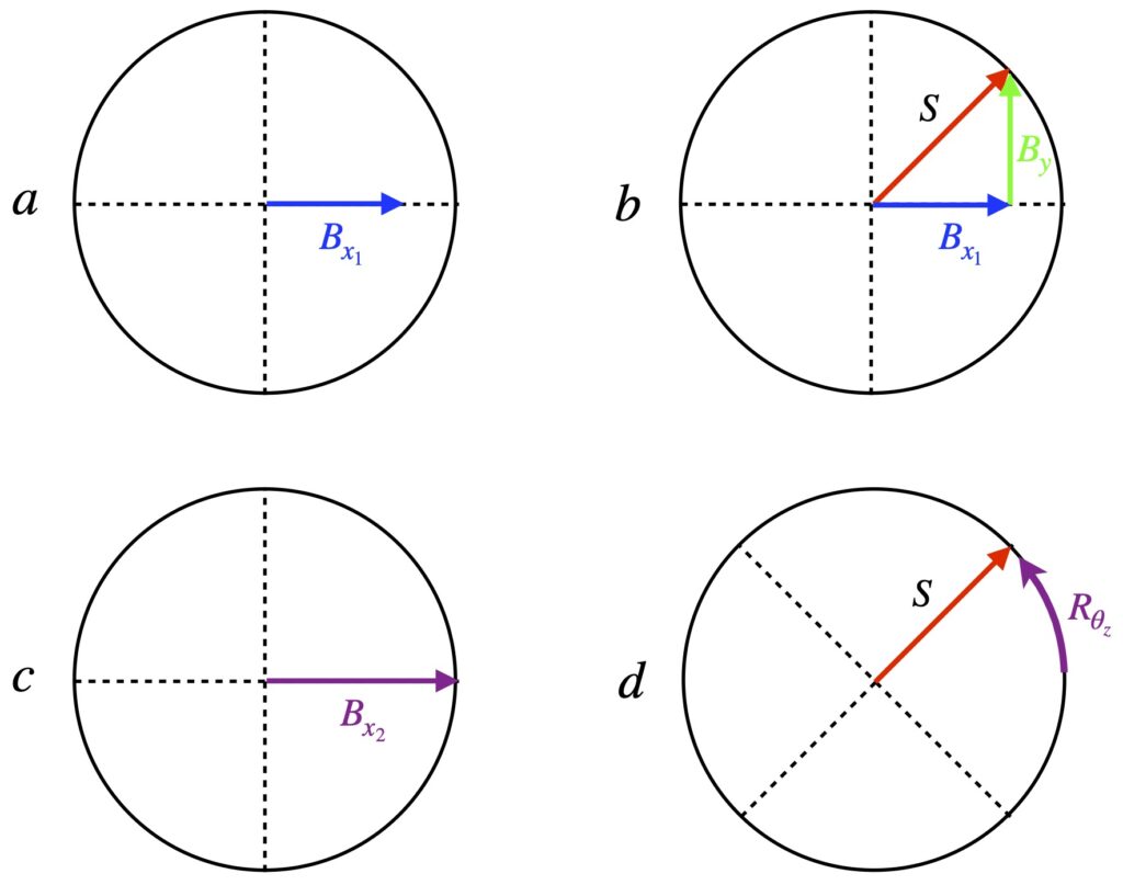
In figure 6.2, it can be seen that a boost in the x-direction,  , followed by a boost in the y-direction,
  leads to vector
  . But so does a larger boost in the x-direction,
  , followed by a rotation around the z-axis,
  . The math that goes along with this gets hairy so I won’t reproduce it here. However, for those who are interested, a detailed mathematical description can be found at https://www.mathpages.com/home/kmath714/kmath714.htm.
The main significance of the Lorentz transformation is that it leaves an entity to which it is applied invariant. This is critical since the ability to do physics depends on its laws being the same in all frames of reference. The concept of invariant quantities is central to special relativity. Therefore, we’ll have much more to say about this concept in the next section.
VII. Invariants in Special Relativity
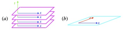
A significant difference between the geometry that governs Newtonian mechanics – Euclidean geometry, the geometry that’s taught in high school – and the geometry that describes special relativity – Minkowski space – is the way time is viewed. This is shown in figure 7.1. In Euclidean space, shown in figure 7.1a, space and time are treated separately. We’re only considering one spatial dimension in figure 7.1a. However, I’ve drawn them on 2-D sheets to convey the idea that, in Euclidean space, “slices of space” progress through time. These slices of space are subject to Galilean relativity but time is considered to be the same in all frames of reference.
By contrast, in Minkowski space, time and space are considered to be on the same footing, as shown in figure 7.1b. In Minkowski space, time and space coordinates depend on each other (per the Lorentz transformation equations) and change in such a way that the speed of light is always constant, in keeping with Einstein’s second postulate.
In both, however, there are entities upon which observers in all frames of reference agree. We’ll call these invariant quantities. In Euclidian geometry, an example of such an invariant is the distance between 2 points in space. Specifically,
![\[ \Delta s ^2= \Delta x ^2 + \Delta y^2 \ \quad \quad \text{eq (7.0.1)} \quad \text{where}\]](https://www.samartigliere.com/wp-content/ql-cache/quicklatex.com-961abf9a12ab93a21d6eb77d2d11adb0_l3.png "Rendered by QuickLaTeX.com")
 is the distance between the 2 points
 is the difference between the x-coordinates at the beginning and end of the line segment formed by the 2 points
 is the difference between the y-coordinates at the beginning and end of the line segment formed by the 2 points
Of course, this is just the well-known Pythagorean theorem.
Figure 7.2 provides an example.
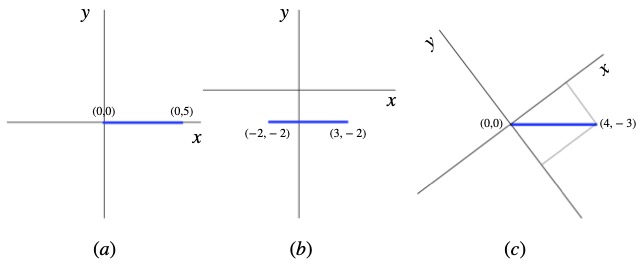
In figure 7.2a, we have a vector that represents the displacement between the points (0,0) and (0,5). The length of this vector is given by :
![\[ \Delta s^2 = (5-0)^2 -(0-0)^2 \quad \Rightarrow \quad \Delta s = \sqrt{25} - 0 = 5 \]](https://www.samartigliere.com/wp-content/ql-cache/quicklatex.com-aefacf0a0ba3e728926693c2a2365d1c_l3.png "Rendered by QuickLaTeX.com")
In figure 7.2b, our coordinate system has been displaced 2 units to upward and 2 units to the right with respect to the coordinate system we used in figure 7.2a. The blue line vector, by eye, looks to be the same length as in figure Xa. Mathematically, we have:
![\[ \Delta s^2 = (3-(-2))^2 + (-2-(-2))^2 \quad \Rightarrow \quad \Delta s = \sqrt{25} - 0 = 5 \]](https://www.samartigliere.com/wp-content/ql-cache/quicklatex.com-2fceb56ada97fef5ce15a4975ec6fa1f_l3.png "Rendered by QuickLaTeX.com")
In figure 7.2c, the axes are rotated counterclockwise compared with those in figure 7.2a. To see that the length of the blue vector is the same as in the first 2 cases takes a little more work. In this case, the vector  is multiplied by the rotation matrix
  to get a new vector
  (where
  , if we measure it, is ~36.87°):
![\[ \begin{pmatrix} x^{\prime}\\y^{\prime}\end{pmatrix} = \begin{pmatrix}\cos (36.87) & \sin (36.87) \\ -\sin (36.87) & \cos (36.87) \end{pmatrix} \begin{pmatrix} 5\\0\end{pmatrix} \]](https://www.samartigliere.com/wp-content/ql-cache/quicklatex.com-9a5f9f47fd10ee9e0b05200395780966_l3.png "Rendered by QuickLaTeX.com")
When we perform the matrix multiplication, we get:
![\[ x^{\prime}=5\cdot \cos(36.87) + 0\cdot \sin (36.87) = 5(0.8) + 0 = 4 \]](https://www.samartigliere.com/wp-content/ql-cache/quicklatex.com-0d58dc590337a893d92f4e6fc55d0859_l3.png "Rendered by QuickLaTeX.com")
and
![\[ y^{\prime}=5\cdot \left(-\sin(36.87)\right) - 0\cdot \cos (36.87) = -5(0.6) + 0 = -3 \]](https://www.samartigliere.com/wp-content/ql-cache/quicklatex.com-e93b2d332b8764467e2ba484cbaf4a48_l3.png "Rendered by QuickLaTeX.com")
We already know the lefthand-most point of the blue vector is at the origin, at (0,0). From our calculations above, the vector ends at the point (4, -3). Putting these values into our equation for  , we obtain:
![\[ \Delta s^2 = (4-0)^2 + (-3-0)^2 \,\,\Rightarrow \,\, \Delta s = \sqrt{16 +9} - 0 = \sqrt{25}-0 = 5 \]](https://www.samartigliere.com/wp-content/ql-cache/quicklatex.com-673b4e7fca7fe5880b2f8c07ea72ddb0_l3.png "Rendered by QuickLaTeX.com")
If desired, you can find further details about the rotation matrix here.
We can make the interval smaller and smaller, until it’s infinitesimal in length. We call this the line element,  where
where
![\[ds^2 = dx^2 + dy^2\quad \quad \text{eq (7.0.2)}\]](https://www.samartigliere.com/wp-content/ql-cache/quicklatex.com-004f32dce056572d64f60f7035cf82e0_l3.png "Rendered by QuickLaTeX.com")
 and
and  being infinitesimal displacements in the x- and y-directions, respectively.
In 3-dimensional space, eq (7.2) becomes:
![\[ds^2 = dx^2 + dy^2 + dz^2 \quad \quad \text{eq (7.0.3)}\]](https://www.samartigliere.com/wp-content/ql-cache/quicklatex.com-6c5676e151f1911be3d88bb4695c61a8_l3.png "Rendered by QuickLaTeX.com")
We need to remember, though, that this only works when the coordinate system has what’s called an orthonormal basis. In general, the length of a vector is given by it’s dot product. Let me explain.
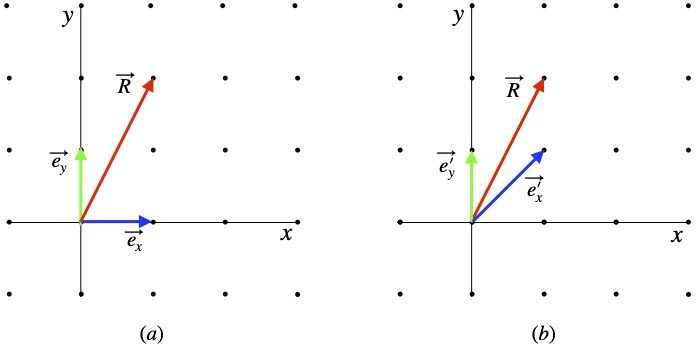
Suppose, as shown in figure 7.3a, we have a Euclidean coordinate system with a column vector  . The 1 and 2 within the parentheses in this vector are just a part of the vector – the components – which represent the magnitude of the vector in a particular direction. The directions, in turn, are given by basis vectors,
  and
and  . The combined vector,
  is:
is:
![\[ \vec{R} = 1\vec{e_x} + 2\vec{e_y} \]](https://www.samartigliere.com/wp-content/ql-cache/quicklatex.com-b9cb3143807c48d2e8fdac0dbae98cc6_l3.png "Rendered by QuickLaTeX.com")
To find the length of , since we’re dealing with an orthonormal basis, we can apply the Pythagorean theorem and it works:
![\[ \lvert R \rvert ^2 = 1^2 + 2^2 = 5 \Rightarrow \lvert R \rvert = \sqrt{5}\]](https://www.samartigliere.com/wp-content/ql-cache/quicklatex.com-602081996cb0bb1eb7761a603378a028_l3.png "Rendered by QuickLaTeX.com")
By the dot product method:

To see why the basis vector dot products are what they are, click .
![\[e_x = \begin{pmatrix}1\\0 \end{pmatrix},\,\, e_y = \begin{pmatrix}0\\1 \end{pmatrix}\]](https://www.samartigliere.com/wp-content/ql-cache/quicklatex.com-6399da56c008e3cf91b9a39d0ca9b185_l3.png "Rendered by QuickLaTeX.com")
![\[e_x \cdot e_x = 1 \cdot 1 + 0 \cdot 0 = 1 \]](https://www.samartigliere.com/wp-content/ql-cache/quicklatex.com-c6d69c2f1d3d2943f9ea7a1930b094a6_l3.png "Rendered by QuickLaTeX.com")
![\[e_x \cdot e_y = 1 \cdot 0 + 0 \cdot 0 = 0\]](https://www.samartigliere.com/wp-content/ql-cache/quicklatex.com-f0db935f86518d45ede1c094a85e4afd_l3.png "Rendered by QuickLaTeX.com")
![\[e_y \cdot e_x = 0 \cdot 1 + 1 \cdot 0 = 0\]](https://www.samartigliere.com/wp-content/ql-cache/quicklatex.com-19c0423a64d04ac0fabedf2938f081cf_l3.png "Rendered by QuickLaTeX.com")
![\[e_y \cdot e_y = 0 \cdot 0 + 1 \cdot 1 = 1\]](https://www.samartigliere.com/wp-content/ql-cache/quicklatex.com-579a7b24b0fdeb3bde8ab49542a36e33_l3.png "Rendered by QuickLaTeX.com")
This result agrees with the result we got by applying the Pythagorean theorem. So far, so good.
Now lets look at figure 7.3b.
In a Euclidean space, the basis vectors are orthonormal – ortho meaning orthogonal, meaning their dot product is 0 (because they are perpendicular to each other) – and normal meaning their length is equal to 1. This is true for the basis vectors in Xa. To see this, take the dot product of and :
![\[ \vec{e_x} \cdot \vec{e_y} = \begin{pmatrix} 1\\0\end{pmatrix} \cdot \begin{pmatrix} 0\\1\end{pmatrix} = 1 \cdot 0 + 0 \cdot 1 = 0 + 0 = 0\]](https://www.samartigliere.com/wp-content/ql-cache/quicklatex.com-5273f8fb68961e5efd063daba6138e9f_l3.png "Rendered by QuickLaTeX.com")
This is not the case with  and
and  :
:
![\[ \vec{e_x}^{\prime} \cdot \vec{e_y}^{\prime} = \begin{pmatrix} 1\\1\end{pmatrix} \cdot \begin{pmatrix} 0\\1\end{pmatrix} = 1 \cdot 0 + 1 \cdot 1 = 0 + 1 = 1\]](https://www.samartigliere.com/wp-content/ql-cache/quicklatex.com-8bcde1e82241a0b4c5834ddd94ece4c3_l3.png "Rendered by QuickLaTeX.com")
In addition, is not normalized (i.e., its length is not equal to 1):
![\[ \lvert \vec{e_x}^{\prime}\rvert^2 = 1^2 + 1^2 = 2; \,\, \Rightarrow \,\, \left( \vec{e_x}^{\prime} \right) = \sqrt{2} \]](https://www.samartigliere.com/wp-content/ql-cache/quicklatex.com-2405a9cfc0bead384f455e2e9ebb643b_l3.png "Rendered by QuickLaTeX.com")
We can see from figure 7.3b that the equation describing the vector  is:
is:
![\[ \vec{R^{\prime}} = 1e_x^{\prime} + 1e_y^{\prime}\]](https://www.samartigliere.com/wp-content/ql-cache/quicklatex.com-9639e05dbf776543adeebe1e10cfb262_l3.png "Rendered by QuickLaTeX.com")
For those who need a quick refresher on vector addition, click .
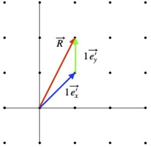

We describe the vectors and in terms of and :
![\[ \vec{e_x}^{\prime} = \vec{e_x} + \vec{e_y} \quad \text{and} \quad \vec{e_y}^{\prime} = \vec{e_y} \]](https://www.samartigliere.com/wp-content/ql-cache/quicklatex.com-28e303b0988cbda704608f20a09edc8e_l3.png "Rendered by QuickLaTeX.com")
So

The vector length-by-dot-product equation becomes:

We can see, from this, that the dot product method of obtaining the length of a vector works in non-orthogonal bases.
In general, the formula for dot product (and thus, for the invariant length, ) can be written as a matrix equation. Here are the details:
![\begin{align*} \vec{R} &= x\vec{e_x} + y\vec{e_y}\\ \lvert R \rvert &= \vec{R} \cdot \vec{R}\\ &= (x\vec{e_x} + y\vec{e_y}) \cdot x\vec{e_x} + y\vec{e_y}\\ &= xx(\vec{e_x} \cdot \vec{e_x}) + xy(\vec{e_x} \cdot \vec{e_y}) + yx(\vec{e_y} \cdot \vec{e_x}) + yy(\vec{e_y} \cdot \vec{e_y})\\ &= \begin{bmatrix} x & y \end{bmatrix} \begin{bmatrix} \vec{e_x} \cdot \vec{e_x} & \vec{e_x} \cdot \vec{e_y}\\ \vec{e_y} \cdot \vec{e_x} & \vec{e_y} \cdot \vec{e_y}\end{bmatrix} \begin{bmatrix} x \\ y \end{bmatrix}\\ &= \begin{bmatrix} x & y \end{bmatrix} \mqty[ g_{xx} & g_{xy} \\ g_{yx} & g_{yy}] \begin{bmatrix} x \\ y \end{bmatrix} \end{align*}](https://www.samartigliere.com/wp-content/ql-cache/quicklatex.com-81922b6978a3194fb60ec34c68f940bc_l3.png "Rendered by QuickLaTeX.com")
VII.1 Spacetime Interval
So what is the spacetime analogue of this invariant in Euclidian space – the length of a vector? It’s the spacetime interval, also an invariant, which we’ll also represent by . But what is it?
Since one of the fundamental postulates of special relativity is the invariance of the speed of light in all reference frames, you might guess that postulate might be the foundation on which the derivation of an invariant quantity in special relativity is built. And you would be correct.
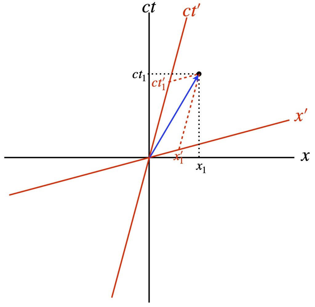
Consider a spacetime diagram (figure 7.1.1.) in which a light beam (blue arrow) traveling from the origin to point  in the x-direction in a frame of reference we’ll call the unprimed frame (black coordinate axes). We know the light beam travels a distance in time so:
![\[ x_1 = c \Delta t_1 \quad \Rightarrow \quad x^2_1 = (c \Delta t_1)^2 \quad \Rightarrow \quad -(c\Delta t_1)^2 + x_1 ^2= 0 \quad \text{eq (7.1.0.1)}\]](https://www.samartigliere.com/wp-content/ql-cache/quicklatex.com-dadc7298e8ab9f3befd4fc9e6120c0e8_l3.png "Rendered by QuickLaTeX.com")
Now, consider a second frame of reference – the primed frame – whose axes are shown in red. We know that the speed of light is the same in all frames of reference. Therefore:
![\[ x_1^{\prime} = c\Delta t_1^{\prime} \quad \Rightarrow \quad x_1^{\prime}^2 = (c \Delta t_1^{\prime} )^2\quad \Rightarrow \quad -(c \Delta t_1^{\prime})^2 + x_1^{\prime}^2 = 0 \quad \text{eq (7.1.0.2)}\]](https://www.samartigliere.com/wp-content/ql-cache/quicklatex.com-ef1deafb1d0cb29e9e66c4b51183dfa9_l3.png "Rendered by QuickLaTeX.com")
Notice that the components of the blue vector representing the world line of the light beam differ for each reference frame i.e.,  versus
  . However, it’s obvious from the diagram these are just different ways of describing the same entity. That is, the spacetime distance traversed by the light beam is invariant.
Note also that, since the expressions on the left side of eq (7.1.0.1) and eq (7.1.0.2) both equal zero, these expressions must be equal to each other:
![\[-(c \Delta t)^2 + x_1^2 = -(c \Delta t^{\prime})^2 + x_1^{\prime}^2 \quad \text{eq (7.1.0.3)}\]](https://www.samartigliere.com/wp-content/ql-cache/quicklatex.com-a213338f9bdd8b5c68e31ca351eb49d5_l3.png "Rendered by QuickLaTeX.com")
And since  for any point
  , we have, in general:
![\[-(c\Delta t)^2 + \Delta x^2 = -(c \Delta t^{\prime})^2 + \Delta x^{\prime}^2 \quad \text{eq (7.1.0.4) for all x}\]](https://www.samartigliere.com/wp-content/ql-cache/quicklatex.com-0944f9d89c0343afd363dfe966057d02_l3.png "Rendered by QuickLaTeX.com")
 , then, is a candidate for an invariant in special relativity. Let’s call it the spacetime interval and give it the same variable name as the length interval in Euclidean geometry, .
Note that, as I’ll discuss later, there are two equally correct conventions for writing the invariant interval in special relativity and the Minkowski metric that’s derived from it. I’ve written the equation  . This leads to one of the conventions. I could’ve written
  as well. This would lead to the other.
At any rate, we know, from what we just said, that  for things traveling at the speed of light (i.e., photons). We’d like, next, to prove that this is true for frames of reference traveling at other speeds.
To do this, we consider events  and
and  occurring in 2 different frames of reference: S and S´, respectively. We know that we can relate these events via the Lorentz transformations.
We start with  and will not use units that result in
  . The Lorentz transformation is:
![\[ c\Delta t^{\prime} = \gamma \left( c\Delta t - \Delta x \frac{v}{c} \right) \quad \text{eq (7.1.0.5) for all x}\]](https://www.samartigliere.com/wp-content/ql-cache/quicklatex.com-531d62ec9388ec5cf27331c9521977cc_l3.png "Rendered by QuickLaTeX.com")
Squaring this equation, recognizing from eq (6.9) that  and doing some algebra, we get:

Next we perform a Lorentz transformation on  :
:
![\[ \Delta x^{\prime} = \gamma \left( -c\Delta t\frac{v}{c} + \Delta x \right) \quad \text{eq (7.1.0.7) for all x}\]](https://www.samartigliere.com/wp-content/ql-cache/quicklatex.com-b44d127c64eaf5d139e9daa4bd0afb53_l3.png "Rendered by QuickLaTeX.com")
Squaring eq (7.1.0.7), using our alternate expression for and doing some more algebra gives us:

Now that we have expressions for  and
and  , we can combine them to get an expression for
  :
:

So  , which is what we wanted to prove i.e.,
  ), the spacetime interval in 2 spacetime dimensions is, indeed, invariant for all coordinate frames involving difference in velocity in the x-direction (so-called x-direction boosts).
We’ve done this for the direction but we can apply this to the  and
and  directions as well to get an invariant in 4D spacetime:
![\[\Delta s^2 = -(c\Delta t)^2 + \Delta x^2 + \Delta y^2 +\Delta z^2 \quad \text{eq (7.1.0.10)} \]](https://www.samartigliere.com/wp-content/ql-cache/quicklatex.com-1e671bf16907c1ebc777ca5345042d71_l3.png "Rendered by QuickLaTeX.com")
The spacetime interval is invariant under rotations of space as well by the following arguments:
- Spatial rotations do not effect time so the
 term should remain unchanged
  is just the length element in Euclidean space which is invariant under rotation
- Since all of the terms on the right side of eq () are invariant,
 , too, must be invariant.
Thus, while observers in different frames of reference may disagree on time and spatial coordinates, all will agree on the separation of spacetime events.
And if we allow all of the elements in eq () to become infinitesimally small, we can come up with an equation that describes the length of infinitesimal distance (or line element) in special relativity:
![\[ds^2 = -ct^2 + dx^2 + dy^2 + dz^2 \quad \text{eq (7.1.0.11)} \]](https://www.samartigliere.com/wp-content/ql-cache/quicklatex.com-502fa8849390a96d8e9a713fdbcfe0cf_l3.png "Rendered by QuickLaTeX.com")
As alluded to above, we can express the length of any vector as its inner (or dot) product with itself, and if that length is infinitesimal, then what we get is the line element. We also said that we could express this line element in a matrix equation. For the space of special relativity, referred to as Minkowski space, the matrix used in such an expression is called the Minkowski metric:
![\[\displaystyle \eta_{\mu \nu} = \displaystyle \begin{bmatrix} g_{00} & g_{01} & g_{02} & g_{03} \\ g_{10} & g_{11} & g_{12} & g_{13} \\ g_{20} & g_{21} & g_{22} & g_{23}\\ g_{30} & g_{31} & g_{32} & g_{33}\end{bmatrix} = \begin{bmatrix} -1 & 0 & 0 & 0\\ 0 & 1 & 0 & 0\\0 & 0 & 1 & 0\\0 & 0 & 0 & 1 \end{bmatrix} \quad \text{eq (7.1.0.12)} \]](https://www.samartigliere.com/wp-content/ql-cache/quicklatex.com-424926c108a245ae6744141bb2a18710_l3.png "Rendered by QuickLaTeX.com")
Following the format I used previously, the matrix equation is:
![\begin{align*} ds^2 &= \begin{matrix} [ct & x & y & z] \\ \,& \,& \,& \,\\ \,& \,& \,& \,\\ \,& \,& \,& \,\\ \end{matrix}\begin{bmatrix} -1 & 0 & 0 & 0\\ 0 & 1 & 0 & 0\\0 & 0 & 1 & 0\\0 & 0 & 0 & 1 \end{bmatrix}\begin{bmatrix} ct \\ x \\ y \\ z\end{bmatrix} \\ \,\\ &= -(ct)^2 + x^2 +y^2 +z^2\\ \,\\ &= \begin{matrix} [x_0 & x_1 & x_2 & x_3] \\ \,& \,& \,& \,\\ \,& \,& \,& \,\\ \,& \,& \,& \,\\ \end{matrix}\begin{bmatrix} -1 & 0 & 0 & 0\\ 0 & 1 & 0 & 0\\0 & 0 & 1 & 0\\0 & 0 & 0 & 1 \end{bmatrix}\begin{bmatrix} x_0 \\ x_1 \\ x_2 \\ x_3\end{bmatrix} \\ \, \\ &= -(x_0)^2 + (x_1)^2 + (x_2)^2 + (x_3)^2 \quad \text{eq (7.1.0.13)} \end{align*}](https://www.samartigliere.com/wp-content/ql-cache/quicklatex.com-a742f547cd2b4cf9b673e284016a99b5_l3.png "Rendered by QuickLaTeX.com")
Notice that, in the lower 2 terms in eq (7.1.0.13), I’ve made the following replacements:

This is standard nomenclature in many texts. We’ll use both the (t, x, y, z) and (x_0, x_1, x_2, x_3) on this page, depending on what best illustrates the point I’m trying to make.
At this point, if the reader has no familiarity with tensors and the Einstein summation convention, it would do well to obtain some knowledge about these topics since they pop up frequently in relativity. For example, eq (7.1.0.13) is often expressed as:

I have a page on this website that gives an introduction to tensors. On that page, I list several additional resources for learning about tensors. Also on my tensor page is a section on the metric tensor. However, for the time being, hopefully readers unfamiliar with these topic will get the gist of eq (7.1.0.14) if I re-write it in the following form:

We know from the line element of the Minkowski metric that the only  terms that are nonzero are the ones where
Therefore, we have:

Here are a few comments about tensors and Einstein summation notation that may be helpful:
- Tensors are categorized according to the number of indices they have; the number of indices a tensor has is called its rank
- Scalars (plain numbers) have 0 indices and are rank 0 tensors; vectors have 1 index and are rank 1 tensors; the metric tensor has 2 indices and is a rank 2 tensor
- Superscripted (upper) indices are referred to as contravariant; Subscripted (lower) indices are referred to as covariant
- When the same upper and lower index appears in a single expression, that index is summed over and yields a scalar
- e.g. Dot product can be written:

- e.g. Dot product can be written:
- Indices that are summed over in an expression can be “cancelled”, kind of like the same number in the numerator and denominator when multiplying 2 fractions
- e.g.
 (a scalar that has no indices) vs.
- e.g.
- Scalars are the same in all coordinate systems. Thus, if we can manipulate terms to create a scalar, that entity will be an invariant
VII.1.1 Spacetime Interval Categories
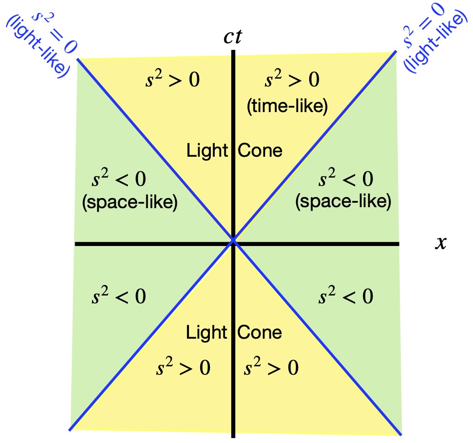
We know that light travels at, well, the speed of light, Light will travel a distance  in the x-direction in per each increment of on the ct axis. Therefore, on a spacetime diagram, the world line of a light beam is represented as a line at a 45° angle (if the light is moving in the +x direction) or a line at 135° (if the light is moving in the -x direction). Light world lines are depicted as blue lines in figure 7.1.1.1. The spacetime interval for a light beam from point (0,0) to (x,ct) is:
![\[ s^2 = (ct)^2 - x^2 \quad \text{eq (7.1.1.1}) \]](https://www.samartigliere.com/wp-content/ql-cache/quicklatex.com-ea14bab4621b1148ad54d8b9da8e8e36_l3.png "Rendered by QuickLaTeX.com")
Here, I’m using the (+,-,-,-) form of the Minkowski metric rather than the the (-,+,+,+) form we’ve used previously simply because it corresponds to what’s shown in figure 7.1.1.1 and figure 7.1.1.1 is the way the following discussion in most often presented. If I had used the (-,+,+,+) convention, then figure 7.1.1.1 would’ve had to have been rotated clockwise 90°.
At any rate, we just said that in time, , the light beam travels a distance . Therefore, the spacetime interval from (0,0) to (x,ct) is zero:
![\[ s^2 = (ct)^2 - x^2 = (ct)^2 - (ct)^2 = 0 \quad \text{eq (7.1.1.2})\]](https://www.samartigliere.com/wp-content/ql-cache/quicklatex.com-fe7a130a20c1295b6deac2f5864ec623_l3.png "Rendered by QuickLaTeX.com")
From this, an object traveling at the speed of light is said to follow a light-like course through spacetime.
On the other hand, if the object’s speed is < c, then  which implies that
  . Therefore,
![\[ s^2 = (ct)^2 - x^2 > 0 \quad \text{eq (7.1.1.3})\]](https://www.samartigliere.com/wp-content/ql-cache/quicklatex.com-c1f09347342ad23d55d597c0f495ab37_l3.png "Rendered by QuickLaTeX.com")
Such objects are said to follow a time-like course through spacetime. Since all objects that we currently know about in physics travel at a speed < c, all known object follow a time-like world lines.
We talked previously about how observers in different frames of reference will consider events to occur at different times. However, for all objects following time-like trajectories (which are all objects that we know of), there is no frame of reference that will change the sequence of events. Which is a good thing because for event A to cause event B, event A has to occur before event B. If we could find a frame of reference where event B occurred before event A, then the effect (event B) would precede the cause (event A), as situation that has never been observed.
Finally, if an object’s speed were > c, then, by the same argument presented above,  . In this case:
![\[ s^2 = (ct)^2 - x^2 < 0 \quad \text{eq (7.1.1.4})\]](https://www.samartigliere.com/wp-content/ql-cache/quicklatex.com-90d16d742b85026556e4f61673e86835_l3.png "Rendered by QuickLaTeX.com")
The world line of such an object is called space-like. Under space-like conditions, frames of reference can be found where sequence of events can be changed, and thus, causality can be “overturned.” Since we don’t think objects can travel with speeds > c, we don’t believe space-like spacetime trajectories exist.
To summarize:


This terminology applies when we use the Minkowski metric of the form (+,-,-,-). If we had used the opposite convention (-,+,+,+), then the categories of the spacetime interval would be:


VII.1.2 Hyperbolic Geometry
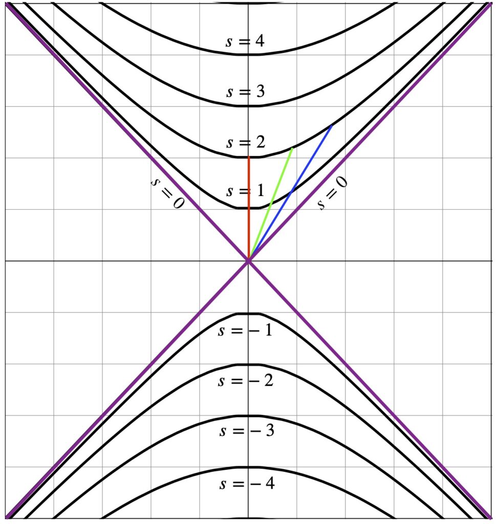
We’ve seen the equation for the spacetime interval in Minkowski space, the spatial geometry where special relativity plays out:
![\[ s^2 = (ct)^2 - x^2 \quad \text{eq (7.1.1.1)} \]](https://www.samartigliere.com/wp-content/ql-cache/quicklatex.com-7bc30faa007a92567c4b98edf01c8b9b_l3.png "Rendered by QuickLaTeX.com")
The graph of these equations are a series of hyperbolae, as depicted in figure 7.1.2.1.
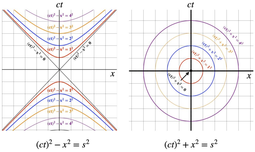
At this point, it’s necessary for the reader to have at least basic familiarity with hyperbolic geometry. A brief introduction to hyperbolic geometry can be found here. However, to gain some intuition as to the meaning of figure 7.1.2.1, let’s compare the equations for a hyperbola and circle:
![\[ \underbrace{(ct)^2 - x^2 = s^2}_{\text{hyperbola}} \quad \text{vs} \quad \underbrace{(ct)^2 + x^2 = s^2}_{\text{circle}} \quad \text{eq (7.1.2.1)} \]](https://www.samartigliere.com/wp-content/ql-cache/quicklatex.com-a0868c17eda368c8d6bad7660c43c446_l3.png "Rendered by QuickLaTeX.com")
In both cases, the quantity  represents a distance from the origin that’s the same. In the case of the circle, equals the circle’s radius and the invariant quantities are represented by concentric circles. With the hyperbola, graphing the invariant “distances” results in the mirror-image boomerang-shaped objects seen in the diagram. The obvious differences in the equations for the hyperbola and circle that create these differing pictures are the minus sign in the hyperbola equation versus the plus sign in the equation for the circle.
Going back to figure 7.1.2.1, we note that the red, green and blue line segments all represent spacetime intervals of 2. They don’t look the same “length” because we’re not dealing with Euclidean space; we’re dealing with Minkowski space which is a different entity. Note that the red line segment is oriented along the vertical time axis and represents an object at rest, moving in time but not in space. The green and blue segments are oriented along time axes for objects in frames of reference that are moving in space with respect to that of the red segment. The speed of the object which the blue line segment represents is moving faster than the object represented by the green segment.
With this background, we’re now ready to see how boosts (Lorentz transformations that relate coordinates moving relative to each other) can be described by rotations in the hyperbolic geometry that underlies Minkowski space.
VII.1.2.1 Lorentz Boosts as Hyperbolic Rotations
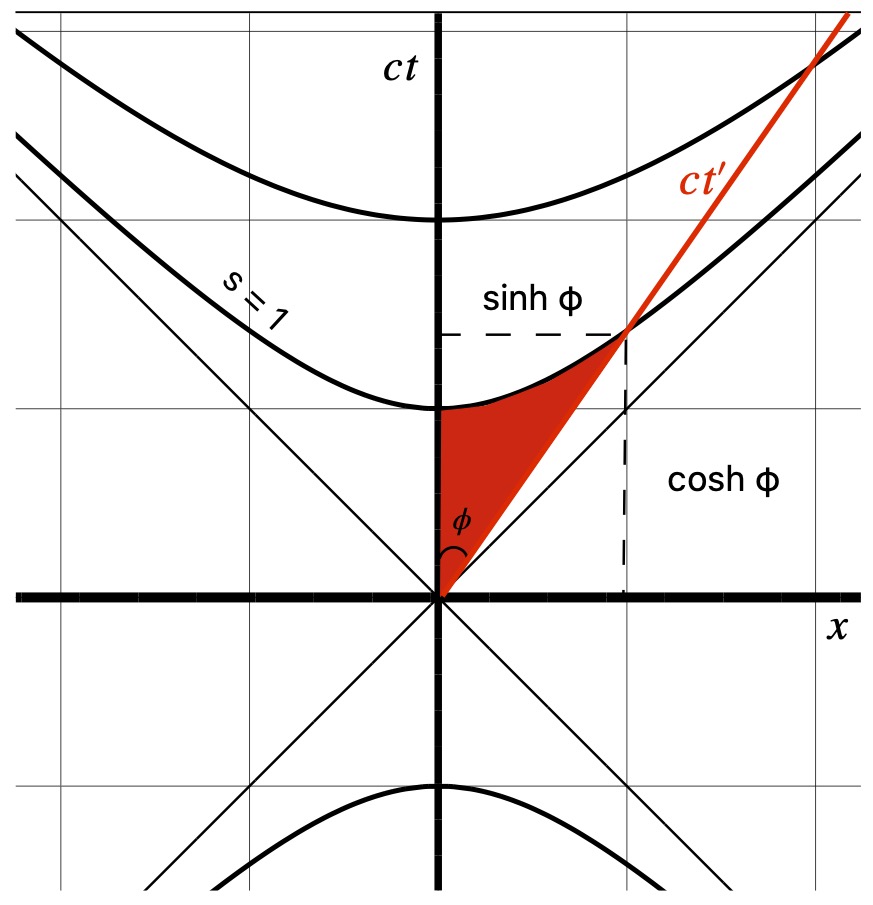
Figure 7.1.2.2.1 shows an invariant hyperbola with  . 2 coordinate systems are pictured:
  and
and  . (The
  is not shown.) We’re looking at things from the nonprimed system’s viewpoint. The primed system is in motion relative to the nonprimed system (at quite high speed, actually). The axis makes a hyperbolic angle,
  , with the axis. Similar to trigonometry in Euclidean space, the point at which the axis intersects the invariant hyperbola is give by the hyperbolic trigonometric functions
  and
and  . And like in Euclidean trigonometry:
![\[\displaystyle \tanh \phi = \frac{\sinh \phi}{\cosh \phi} \quad \text{eq (7.1.2.1.1)} \]](https://www.samartigliere.com/wp-content/ql-cache/quicklatex.com-ce06638079456a1221224543e1d2ad58_l3.png "Rendered by QuickLaTeX.com")
From the diagram, we can see that  and
and  . Therefore:

Next, let’s go back to the equations we derived for the Lorentz transformation in matrix form. I’ll reproduce it here except I’ll call the time axes and instead of and . I’ll also follow the lead of many authors and define:


We end up with:


We can write these equations in matrix form:
![\[ \begin{pmatrix} ct^{\prime}\\ x^{\prime} \end{pmatrix} = \begin{pmatrix} \gamma & -\gamma \beta \\ -\gamma \beta & \gamma \end{pmatrix} \begin{pmatrix} ct\\ x \end{pmatrix} \quad \quad \,\text{eq (7.1.2.1.7)}\]](https://www.samartigliere.com/wp-content/ql-cache/quicklatex.com-1e2f68e8b44f807b601d5252046a4e4c_l3.png "Rendered by QuickLaTeX.com")
and
![\[ \begin{pmatrix} ct\\ x \end{pmatrix} = \begin{pmatrix} \gamma & \gamma \beta \\ \gamma \beta & \gamma \end{pmatrix} \begin{pmatrix} ct^{\prime}\\ x^{\prime} \end{pmatrix} \quad \quad \,\text{eq (7.1.2.1.8)}\]](https://www.samartigliere.com/wp-content/ql-cache/quicklatex.com-c7d80a997c49dc4d0ca40456947e88f4_l3.png "Rendered by QuickLaTeX.com")
Now we need to ask, Can we express and  in terms of hyperbolic trigonometric function? Happily, the answer is yes. We know that:
![\[ \tan \phi = \frac{v}{c} = \beta \quad \,\text{eq (7.1.2.1.9)}\]](https://www.samartigliere.com/wp-content/ql-cache/quicklatex.com-04af000aa92da6326126783b97d81d47_l3.png "Rendered by QuickLaTeX.com")
Therefore:

Similar to  and
and  :
:
![\[ \frac{1}{\sqrt{1 - \tanh^2 \phi}} = \frac{1}{\sqrt{\sech^2 \phi}} = \frac{1}{\sech \phi} = \cosh \phi \quad \,\text{eq (7.1.2.1.11)}\]](https://www.samartigliere.com/wp-content/ql-cache/quicklatex.com-26c63228834da83b5f2dc004395ce817_l3.png "Rendered by QuickLaTeX.com")
So:
![\[ \gamma = \cosh \phi \quad \,\text{eq (7.1.2.1.12)} \]](https://www.samartigliere.com/wp-content/ql-cache/quicklatex.com-8dcd02da650c7bd3c19e8cef175f179f_l3.png "Rendered by QuickLaTeX.com")
Then:
![\[ \gamma \beta = \cosh \phi \tanh \phi = \cancel{\cosh \phi}\frac{\sinh \phi}{\cancel{\cosh \phi}} = \sinh \phi \quad \,\text{eq (7.1.2.1.13)}\]](https://www.samartigliere.com/wp-content/ql-cache/quicklatex.com-7bd7fe06af3ae00a6f96c67ff5b19836_l3.png "Rendered by QuickLaTeX.com")
Substituting these values into matrix equations eq (7.1.2.1.7) and eq (7.1.2.1.8), we get:
![\[ \begin{pmatrix} ct^{\prime}\\ x^{\prime} \end{pmatrix} = \begin{pmatrix} \cosh \phi & -\sinh \phi \\ -\sinh \phi & \cosh \phi \end{pmatrix} \begin{pmatrix} ct\\ x \end{pmatrix} \quad \quad \,\text{eq (7.1.2.1.14)}\]](https://www.samartigliere.com/wp-content/ql-cache/quicklatex.com-9ceb4bc860d2b8af1176d715ca7003fe_l3.png "Rendered by QuickLaTeX.com")
and
![\[ \begin{pmatrix} ct\\ x \end{pmatrix} = \begin{pmatrix} \cosh \phi & \sinh \phi\\ \sinh \phi & \cosh \phi \end{pmatrix} \begin{pmatrix} ct^{\prime}\\ x^{\prime} \end{pmatrix} \quad \quad \,\text{eq (7.1.2.1.15)}\]](https://www.samartigliere.com/wp-content/ql-cache/quicklatex.com-e29a9434b79629b48dbf84243a28fa00_l3.png "Rendered by QuickLaTeX.com")
The matrices
![\[\begin{pmatrix} \cosh \phi & -\sinh \phi \\ -\sinh \phi & \cosh \phi \end{pmatrix}\quad \text{and} \quad \begin{pmatrix} \cosh \phi & \sinh \phi\\ \sinh \phi & \cosh \phi \end{pmatrix}\quad \,\text{eq (7.1.2.1.16)}\]](https://www.samartigliere.com/wp-content/ql-cache/quicklatex.com-f1318c34a9b1a7e95a5a386a4f228994_l3.png "Rendered by QuickLaTeX.com")
resemble the Euclidean rotation matrix and its inverse:
![\[ \begin{bmatrix}\,\,\,\,\cos\theta&\sin\theta\\-\sin\theta&\cos\theta\end{bmatrix} \quad \text{and} \quad \begin{bmatrix}\cos \theta & -\sin \theta\\ \sin \theta & \cos \theta \end{bmatrix}\quad \,\text{eq (7.1.2.1.17)} \]](https://www.samartigliere.com/wp-content/ql-cache/quicklatex.com-455f65d23ad9e6097aef57dedcff6785_l3.png "Rendered by QuickLaTeX.com")
Thus, the matrices shown in eq (7.1.2.1.16) are usually referred to as hyperbolic rotation matrices.
However, the geometric meaning of hyperbolic rotations are decidedly different than rotations in Euclidean space.
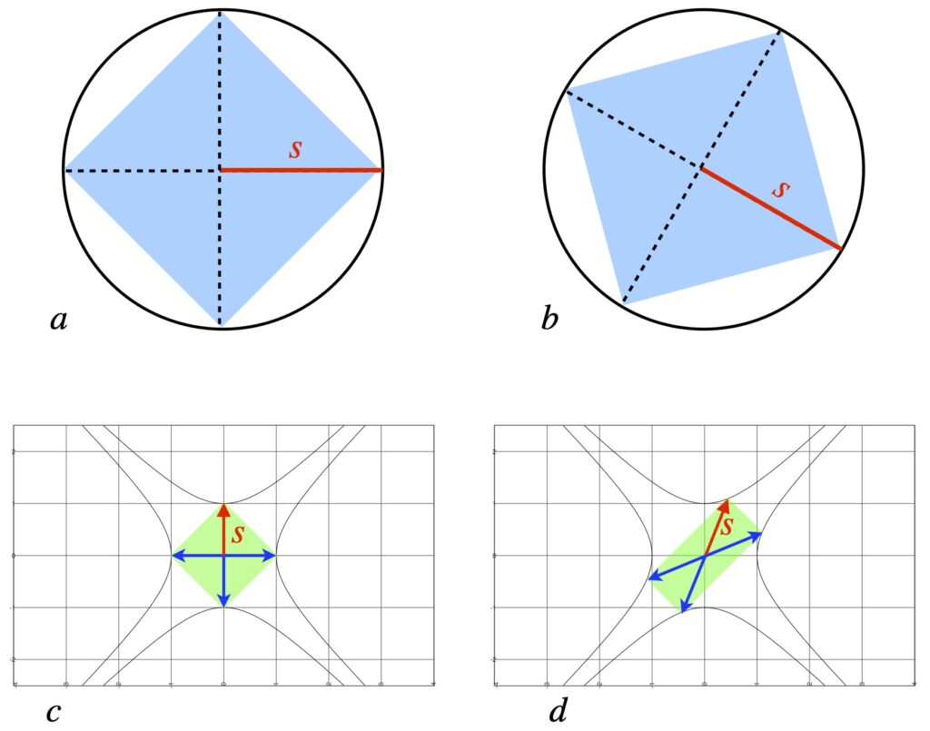
Figure 7.1.2.2.2a shows a polar coordinate system in Euclidean space containing a red vector with the length, s, equal to the radius of a circle. is an invariant in Euclidean space (i.e.,  . Line segments connecting points on the circle to ends of the coordinate axes form a blue square.
Figure 7.1.2.2.2b depicts a clockwise rotation of the the coordinate axis. Note that the radius, , remains the same. Also, the area of the square also remains unchanged (i.e., it’s the same square; it’s just rotated).
Figure 7.1.2.2.2c and figure 7.1.2.2.2d represent Minkowski space. Unit hyperbolae represent invariant “surfaces” with  . In figure 7.1.2.2.2c, the green box contains blue axes and a red vector with “length” of . Figure 7.1.2.2.2d depicts a hyperbolic rotation. In contrast to the Euclidean rotation, the green box changes shape (elongates in one direction and narrows in the other). However, its area and the invariant quantity, , remain unchanged. Note that the coordinate axes in the green box “scissor together” as a result of the hyperbolic rotation. Of course, we’ve already seen that relative motion due to a velocity boost also yields coordinate axes that scissor together, again indicating the equivalence of the Lorentz boost and hyperbolic rotation.
Note also that the determinants of both the Euclidean and hyperbolic rotation matrices equals 1, and the determinant represents the area of the blue and green polygons reflecting the invariant nature of these operations. For more information about the determinant and its geometric interpretation, click here.
VII.1.2.2 Velocity Addition
I’ve waited until now to introduce the relativistic velocity formula for reasons that will become apparent soon. We’ll start with the standard derivation of velocity addition then look at it from the perspective of hyperbolic geometry.
This derivation is taken from Khan Academy although it’s similar to derivations found elsewhere.
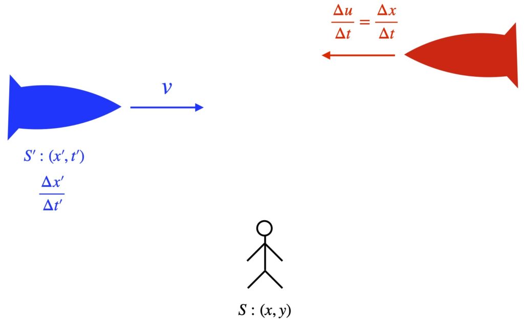
In figure 7.1.2.2.1, we have an observer, floating in space, in frame of reference , with spatial coordinates  . This observer sees a blue rocket moving to the right at relativistic speed . We’ll call the blue rocket’s frame of reference and its coordinates
  . There’s also a red rocket moving to the left with velocity
  in the frame. What we want to find out is the velocity,
  , seen in the frame.
We start by writing the terms  and in terms of the frame of reference coordinates using the Lorentz transformation:

and
![\[ \Delta t^{\prime} = \gamma(\Delta t - \frac{v}{c^2}) \Delta x ) \quad \text{7.1.2.2.2} \]](https://www.samartigliere.com/wp-content/ql-cache/quicklatex.com-76bc4781f1f0078b51e1f0029c7df731_l3.png "Rendered by QuickLaTeX.com")
To get the velocity in the frame, we divide eq (7.1.2.2.1) by eq (7.1.2.2.2), then do some algebra:

But . So:
![\[ \frac{\Delta x^{\prime}}{\Delta t^{\prime}} = \frac{\displaystyle \frac{\Delta u}{\Delta t}-v}{1 - \displaystyle \frac{v}{c^2}\cdot\displaystyle \frac{\Delta u}{\Delta t}} \quad \text{7.1.2.2.4} \]](https://www.samartigliere.com/wp-content/ql-cache/quicklatex.com-2c812a949ba77e994927f9d62545daa1_l3.png "Rendered by QuickLaTeX.com")
Now we take the limit as  :
:
![\[ \lim_{\Delta t \rightarrow 0} \frac{\Delta x^{\prime}}{\Delta t^{\prime}} = v^{\prime} = \displaystyle \frac{u-v}{1-\displaystyle \frac{uv}{c^2}} \quad \text{7.1.2.2.5} \]](https://www.samartigliere.com/wp-content/ql-cache/quicklatex.com-bf9cdf106a5ed75c4db4abc2a8b05bda_l3.png "Rendered by QuickLaTeX.com")
Notice that  is just the Galilean velocity addition rule. In special relativity, this is modified by the factor
  .
.
We can put in some numbers to better understand how this works. Suppose the blue rocket is moving to the right at  and the red rocket is moving to the left at
  . What is the velocity of the red rocket as seen by the observer in the blue rocket (
 )? In Galilean relativity, this would be
  . Of course, far as we know, this is impossible since nothing has ever been observed to move faster than the speed of light. However, when we apply special relativity, we get:

Relativistic velocity addition can also be achieved using hyperbolic geometry. Recall:
Figure 7.1.2.2.2 shows a graph of  .
.
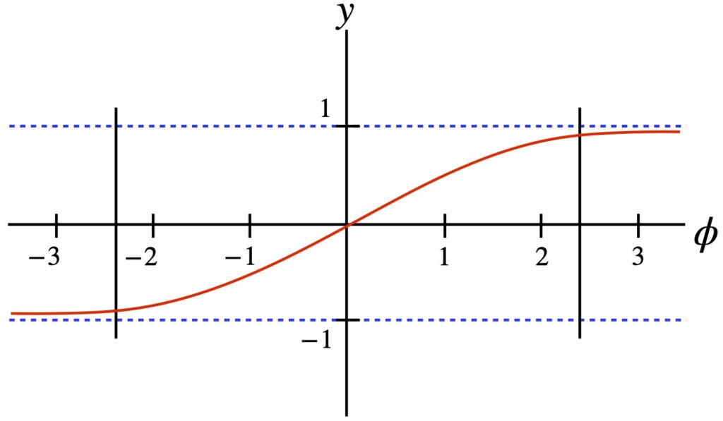
We can see from this graph:
- Unlike Euclidean geometry, where angles of a circle repeat after
 radians, goes to infinity in both the + and – directions.
 - As goes to
 ,
,  approaches
  asymptotically (i.e., tanh gets close to but never reaches y=1). This makes sense since
  , and as we know, massive objects can get close to but never equal .
Figure 7.1.2.2.3 is designed to help illustrate how this works.
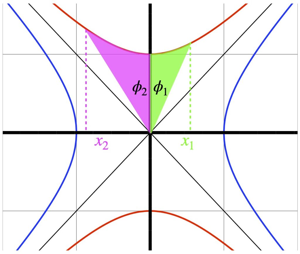
In figure 7.1.2.2.3:
- The red curves represent “unit” invariant hyperbolae where
 .
. - The blue curves are “unit” invariant hyperbolae where
 .
. - The 45° and -45° diagonal black lines represent the paths of light rays.
- The right hand margin of the green “hyperbolic triangle” represents the ct-axis of the blue spaceship traveling in the +x-direction in figure 7.1.2.2.1. It makes a hyperbolic angle of
 with the ct-axis of frame of reference in figure 7.1.2.2.1. is referred to as the rapidity. Looking back at eq (7.1.2.1.2), since we’re working with a unit hyperbola,
  so
so  .
. - Likewise, the lefthand margin of the magenta “hyperbolic triangle” represents the ct-axis of the red spaceship traveling in the -x direction in figure 7.1.2.2.1. It makes a hyperbolic angle of
 with the ct-axis of frame of reference in figure 7.1.2.2.1. And per the same rationale as we just used,
In equation 7.1.2.2.5, we have an equation for velocity addition in special relativity:
![\[ v^{\prime} = \displaystyle \frac{u-v}{1-\displaystyle \frac{uv}{c^2}} \]](https://www.samartigliere.com/wp-content/ql-cache/quicklatex.com-8dde447adcdef671bc1f54b46a67483a_l3.png "Rendered by QuickLaTeX.com")
Divide both sides of this equation by :
![\[ \displaystyle \left(\frac{v^{\prime}}{c}\right) = \displaystyle \frac{\displaystyle \left(\frac{u}{c}\right)-\displaystyle \left(\frac{v}{c}\right)}{1-\displaystyle \left(\frac{u}{c}\right)\displaystyle \left(\frac{v}{c}\right)} \quad \text{eq (7.1.2.2.6)} \]](https://www.samartigliere.com/wp-content/ql-cache/quicklatex.com-7012a92881882db650d6615d408a37ac_l3.png "Rendered by QuickLaTeX.com")
But:


Substituting these values into eq (7.1.2.2.6) gives us:
![\[ \displaystyle \tanh \phi_{v^{\prime}} = \displaystyle \frac{\tanh \phi_{u} -\tanh \phi_{v}}{1-\displaystyle \left(\tanh \phi_{u}\right)\displaystyle \left(\tanh \phi_{v}\right)} \quad \text{eq (7.1.2.2.10)} \]](https://www.samartigliere.com/wp-content/ql-cache/quicklatex.com-0c389e00d5d245a47363ea2cb848a65d_l3.png "Rendered by QuickLaTeX.com")
However, eq (7.1.2.2.10) is just the hyperbolic tangent sum formula:
![\[ \displaystyle \tanh (\phi_{u} + \phi_{v}) = \displaystyle \frac{\tanh \phi_{u} -\tanh \phi_{v}}{1-\displaystyle \left(\tanh \phi_{u}\right)\displaystyle \left(\tanh \phi_{v}\right)} \quad \text{eq (7.1.2.2.11)} \]](https://www.samartigliere.com/wp-content/ql-cache/quicklatex.com-5d8eb1111a174ce692717fb1a349968e_l3.png "Rendered by QuickLaTeX.com")
(For a proof of this formula, click here.)
This means that the hyperbolic angles  ,
,  and
and  (referred to rapidities) are additive:
![\[ \phi_{v^{\prime}} = \phi_u + \phi_v \quad \text{eq (7.1.2.2.12)} \]](https://www.samartigliere.com/wp-content/ql-cache/quicklatex.com-6e8b93c174e353ec16956b42d34b4f4f_l3.png "Rendered by QuickLaTeX.com")
We can apply these formulas to the problem we solved previously and compare the solutions. We’re given that:

Therefore:

Similarly:
![\[v = 0.7c \,\, \Rightarrow \,\,\displaystyle \frac{v}{c}=\displaystyle \frac{0.7c}{c}=0.7\]](https://www.samartigliere.com/wp-content/ql-cache/quicklatex.com-d9779f592ed55b088256d885b2e3f748_l3.png "Rendered by QuickLaTeX.com")
Therefore:
![\[\tanh \phi_v = 0.7 \,\, \Rightarrow \,\, \phi_v = \text{arctanh}(0.7) = 0.8673\]](https://www.samartigliere.com/wp-content/ql-cache/quicklatex.com-4a1679849c680b9648b11a7eea0e7f63_l3.png "Rendered by QuickLaTeX.com")
Then:

This implies that
![\[ \frac{v^{\prime}}{c} = 0.8889 \,\, \Rightarrow \,\, v^{\prime} = 0.8889c \]](https://www.samartigliere.com/wp-content/ql-cache/quicklatex.com-9480751bf6a590c086fc5e68bb0fe285_l3.png "Rendered by QuickLaTeX.com")
which is the same result we got from our other method of calculation.
VII.2 Proper Time
Proper time,  is defined as the time an observer measures in their own frame of reference. We know that in their own frame of reference, observers don’t think they’re moving. Therefore, in their own from of reference,
  and
and  . Plugging these values into our equation for the spacetime interval, we get:

Which implies that:

And since is invariant,  is also invariant. -1 and
  are constants so
  is invariant, and thus,
  is invariant.
VII.2.1 Twin Paradox
This discussion is adapted from Dr. John Simonetti, Dept. of Physics, Virginia Tech University, Frequently Asked Questions About Special Relativity – The Twin Paradox, 21 Oct, 1997.
Imagine twins Alice and Bob. Alice remains on earth while Bob makes a trip to a distant planet and back (figure 7.2.1.1). Since Bob is in a moving frame of reference, Alice sees Bob’s clock as ticking slower than hers. According to her, less time has elapsed for Bob during his trip. Therefore, she expects that Bob will be younger than her when he gets back. However, in special relativity, every frame of reference is equally valid. Thus, Bob, in his frame of reference sees himself at rest and the earth and distant planet as moving. Since Bob considers Alice to be in a moving frame of reference. He sees her clock as ticking slower than his, and thus, less time elapsing for Alice than for him during his trip. When he returns to earth, then, he expects that she will be younger than he is. But how can both twins, Alice and Bob, be older than the other at the same time. This seems to be a contradiction. Actually, it isn’t. Here’s why.
For convenience, let’s change the names of our twins to Unprime and Prime. Obviously, to start motion, stop motion and change directions, Prime must accelerate. Thus, technically, Prime’s frame of reference is not inertial so special relativity doesn’t apply. However, for purposes of this discussion, we’ll assume that acceleration is instantaneous so we don’t have to account for it in our time calculation. We’ll take out acceleration altogether later, but it’ll easier to understand the argument I’m about to make if we consider duration of accelerations to be negligible. Also, to make things more comprehensible, we’ll put in some numbers. Specifically, we’ll say that, according to Unprime, Prime moves at a velocity of v = 0.8c and the distant planet, Planet A, is a distance L = 1 light-year away. Now let’s consider how Unprime and Prime view 3 different events:
- At the start of the experiment
- When Prime reaches Planet A
- At the finish when Prime is back on Earth
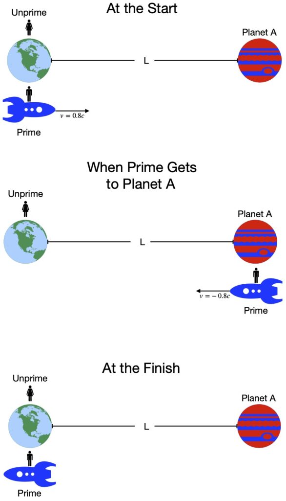
Unprime’s Observations
At the Start
At the start of our experiment, Unprime and Prime synchronize their watches. Unprime says that her clock reads  and Prime says that his clock reads
  . Unprime then sees Prime speed off toward Planet A at
  .
.
When Prime Reaches Planet A
A clock on Planet A, which is at rest in Unprime’s frame, measures  . A photo is taken of this clock reading and sent, at the speed of light, to Unprime.
At Planet A, Prime takes a photo of his clock and transmits it to Unprime. The clock reads  . This is because Unprime sees Prime’s clock as running slowly. Specifically,

where

so

At the Finish
When Prime arrives home, Unprime looks at his clock and notes that it reads  . This is because, if it took 1.25 years for Prime to get to Planet A, and Prime travels the same distance back, at the same speed, then, to Unprime, the time of Prime’s return trip must be the same as his outbound trip. Thus, total time = 1.25 + 1.25 = 2.5.
Unprimed looks at Prime’s clock and notes that it reads  . She is not surprised since she received the photo of Prime’s clock on Planet A which read . Because Prime traveled the same distance, at the same velocity, on his return trip as he did on his outbound trip, Unprime reasons that the return trip must also have taken 0.75 years and that the entire trip, as measured by Prime’s clock, must have taken 1.5 years.
Ultimately, the reason Unprime observes a longer time for the trip than Prime is that Prime’s clock ticked slower due to time dilation.
Prime’s Observations
At the Start
Prime, like Unprime, measures the time at the beginning of the experiment as zero (i.e. and  . Then Prime sees Unprime whizz off away from him at a velocity of
  and Planet A whizz toward him at .
When Prime Reaches Planet A
Or should I say, when Planet A reaches Prime. When it does, Prime notes that his clock measures  . Why, because Planet A is moving relative to Prime, and therefore, due to length contraction, Prime sees the distance Planet A travels as:

He sees the time his clock measured for Planet A to reach him as:

Then Prime looks at the clock on Planet A so he can take a photo of it and send it back to Unprime on earth. He’s initially puzzled to find that the clock on Planet A measures  . Then he remembers his special relativity and comes up with the following explanation:
While Unprime sees her clock as synchronized with the clock on Planet A, Prime does not. While Prime sees his clock as reading at the start of his journey (as does Unprime), to Prime, Planet A has instantaneously accelerated to a velocity of 0.8c. Thus, from the Lorentz transformation, he knows that the clock on Planet A reads something different. Specifically:

To get the time he will read on Planet A’s clock when the planet gets to him, Prime knows that he must add the time that he sees Planet A as taking to reach him to Planet A’s clock’s initial reading that we just calculated:
![\[t_{\text{PlanetAatPrime}} = t_{\text{PlanetAtoPrime}} + t_{\text{PlanetAInitial}}\]](https://www.samartigliere.com/wp-content/ql-cache/quicklatex.com-a8e474eb039fefba50f82db790c8e43a_l3.png "Rendered by QuickLaTeX.com")
The time it takes for Planet A to get to prime is the length it has to travel divided by the velocity at which it travels. But we have to
1) adjust the distance between Prime and Planet A for length contraction i.e., Planet A is moving with respect to Prime so Prime sees the distance Planet A travels as:
![\[L^{\prime}=\frac{L}{\gamma} \]](https://www.samartigliere.com/wp-content/ql-cache/quicklatex.com-2dde3db862fb7be5d1dd9143d54cef61_l3.png "Rendered by QuickLaTeX.com")
From this, we might expect that the travel time for Planet A to Prime is:
![\[ t_{\text{PlanetAtoPrime}} = \frac{L^{\prime}}{v} = \frac{L/ \gamma}{v} \]](https://www.samartigliere.com/wp-content/ql-cache/quicklatex.com-98d35fe29a8ed23943a596ce923828d5_l3.png "Rendered by QuickLaTeX.com")
However, we also need to:
2) adjust Planet A’s travel time for time dilation i.e., Planet A is moving with respect to Prime, so Prime sees the planet’s actual travel time as:
![\[ t_{\text{PlanetToPrime}} = \frac{L^{\prime}/v}{\gamma} = \frac{(L/ \gamma)/v}{\gamma} = \frac{L}{v} \cdot \frac{1}{\gamma^2}\]](https://www.samartigliere.com/wp-content/ql-cache/quicklatex.com-132934cab6f8ab6793ea9e8f15d7b303_l3.png "Rendered by QuickLaTeX.com")
So

But  . Thus,
  and therefore,

Of course, 1.25 years is exactly what Planet A’s clock measured in Unprime’s frame. And 0.75 years, the time Prime measures at Planet A, is exactly the time that Unprime saw Prime’s clock measuring in her frame of reference.
At the Finish
When planet Earth (with Unprime on it) reaches prime, Prime’s clock measures , as he expected since it took 0.75 years for the planet to reach him, and Earth’s/Unprime’s velocity traveling toward him is the same as Planet A’s speed. Therefore, the degree of time dilation Prime sees is the same as that which affected the time he observed when Planet A traveled to him.
Next, Prime looks at Unprime’s clock when Earth “re-reaches” him and sees that it measures  . To explain this, he makes an argument similar to the one he used to find the time it took for Planet A to get to him.
Prime reasons that when the Earth (and Unprime) start their journey toward him, the clock on the planet and Unprime’s clock are not synchronized, for the same reason Prime’s and Planet A’s clocks are not synchronized at the start of the experiment. Unprime’s clock on Earth reads  years more than the clock on Planet A at the start of Unprime’s trip back to Prime. And the time, according to Prime, for Unprime to reunite with him is the length of the trip adjusted for length contraction, divided by the velocity of Earth/Unprime, all adjusted for the time dilation brought about by the Earth’s/Unprime’s motion relative to Prime, plus . That is, it’s the same as the time interval measured after Planet A makes its trip to Prime: 1.25 years.
Thus, the total time for Planet A to get to Prime (who’s at rest in his own frame of reference) and the Earth/Unprime to return to Prime is 1.25 + 1.25 = 2.5 years, the same as the time Unprime measures for Prime to travel to and back from Planet A. This is due to a combination of time dilation and the relativity of simultaneity. In short, there is no paradox. Both Unprime and Prime agree that Prime is younger when he comes back to Earth after his journey.
It’s been said that it’s the acceleration experienced by Prime that somehow makes him age less than his twin sister. However, we can redo the above example without acceleration and get the same result. Here’s how:
Imagine Unprime sitting on Earth with a clock. Prime rushes by Unprime, on a rocket, moving at relative to Unprime. The rocket, for as long as we know about, has been moving at that constant velocity v. When Prime reaches Unprime, they both set their clocks to zero. Prime travels on to, then past, Planet A. At Planet A, Prime looks at his clock and notes that it reads 0.75 years, due to length contraction.
At the exact time Prime reaches Planet A, another observer, Doubleprime, flies by at a velocity  relative to Unprime. For as long as we know, Doubleprime has been moving at this velocity. As he passes Prime, he and Prime set their clocks to t = 0.75 years. Doubleprime continues on towards earth, then past. At the moment Doubleprime passes Unprime, they look at their clocks. They both note that Doubleprime’s clock reads 1.25 years and Unprime’s reads 2.5 years. Unprime’s explanation for the difference is time dilation and Doubleprime’s explanation is time dilation and lack of clock synchronization, just like in the example above with acceleration.
The difference in clock measurements by Doubleprime and Unprime in the latter example are not the result of acceleration (there is none in this example). Rather, it’s due to the fact that the entire experiment takes place in one inertial frame of reference for Unprime but requires two inertial frames of reference for Doubleprime (and for Prime in the previous example).
Another way to look at the reason for this difference is given by eignchris, beginning at 12:05 of his YouTube video, Relativity 105d: Acceleration – Twin Paradox and Proper Time Along Curves (Rindler Metric).
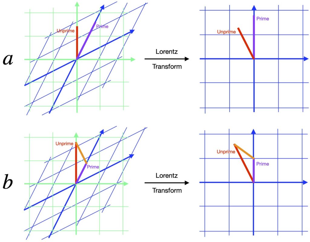
The video’s author points out that, to transform between two worldlines in special relativity, one must apply a Lorentz transformation. The assumption that leads to the twin paradox is that we can transform 1) the worldline corresponding to a frame of reference in which Unprime is at rest into 2) one where the worldline corresponds to a frame of reference in which Prime is at rest. The problem is that Prime’s worldline consists of two inertial frames of reference, a frame of reference eigenchris refers to as a “zigzag worldline.” And as eigenchris points out, a Lorentz transformation cannot “straighten out” a zigzag world line (i.e., make the entire worldline follow the course of the spacetime time axis, the type of worldline required to represent a body at rest).
VII.3 4-Velocity
This derivation is adapted from Collier, Peter. “Special Relativity.” A Most Incomprehensible Thing: Notes Towards a Very Gentle Introduction to the Mathematics of Relativity, Incomprehensible Books, 2019, pp. 119-121. This book can be found on Amazon at https://www.amazon.com/Most-Incomprehensible-Thing-Introduction-Mathematics/dp/0957389469
Consider an object moving through 3D space. The path of the object can be parameterized with each of the spatial coordinates being functions of time:

We can find the velocity in each direction of space at each time by differentiating and multiplying by the basis vector in each spatial direction:
![\[V(t) = \frac{dx}{dt}\vec{e}_x + \frac{dy}{dt}\vec{e}_y + \frac{dz}{dt}\vec{e}_z \quad \text{eq (7.3.2)} \]](https://www.samartigliere.com/wp-content/ql-cache/quicklatex.com-e6c87306e10864eb7bb4b672ff4b2a8b_l3.png "Rendered by QuickLaTeX.com")
Notice that what we consider the “normal” velocities are components of a vector, not the vector itself. And we know that vector components usually vary with coordinate transformations (whereas the entire vector does not). Therefore, regular everyday velocities are not invariants in special relativity. However, we can create a velocity vector that is form-invariant. We do this by defining an entity called the 4-velocity which consists of the rate of change in each coordinate “direction” in special relativity (t, x, y and z =  , respectively) with respect to proper time (which we know is invariant). Thus:
![\[U^u = \displaystyle \frac{dx^u}{d\tau} = \left(c\frac{dx^t}{d\tau},\, \frac{dx^t}{d\tau},\, \frac{dy^t}{d\tau},\, \frac{dz^t}{d\tau}\right) \quad \text{eq (7.3.3)} \]](https://www.samartigliere.com/wp-content/ql-cache/quicklatex.com-161b3dd3e5be3b7aefed938ddce85edf_l3.png "Rendered by QuickLaTeX.com")
From our discussion of time dilation, we know that:
![\[ \Delta t = \gamma \Delta \tau \quad \text{eq (7.3.4)} \]](https://www.samartigliere.com/wp-content/ql-cache/quicklatex.com-4c434f6f39a4251c3fa798bd1e24d662_l3.png "Rendered by QuickLaTeX.com")
That means:
![\[ x^0 = ct = c\gamma \tau \quad \text{eq (7.3.5)} \]](https://www.samartigliere.com/wp-content/ql-cache/quicklatex.com-781d6d3ae36938a853fd5ee104b941b9_l3.png "Rendered by QuickLaTeX.com")
Taking the derivative with respect to proper time gives:
![\[ U^0 = \displaystyle \frac{dx^0}{d\tau} = c\gamma \quad \text{eq (7.3.6)} \]](https://www.samartigliere.com/wp-content/ql-cache/quicklatex.com-1b8f3eccf5c2e9993ae209940861c5bb_l3.png "Rendered by QuickLaTeX.com")
Using the chain rule for the spatial components:
![\[ U^i = \displaystyle \frac{dx^i}{dx^0}\frac{dx^0}{d\tau} = \frac{dx^i}{dx^0}c\gamma = \frac{dx^i}{dx(ct)}c\gamma = \frac{dx^i}{cdt}c\gamma = \frac{dx^i}{dt}\gamma \quad \text{eq (7.3.7)} \]](https://www.samartigliere.com/wp-content/ql-cache/quicklatex.com-58f6574a510048df93291f32c77c0e1c_l3.png "Rendered by QuickLaTeX.com")
 is the regular spatial velocity where
![\[\displaystyle \vec{v} = \left( \frac{dx^1}{dt}, \frac{dx^2}{dt}, \frac{dx^3}{dt}, \right) = (v_x,\, v_y\, v_z) \quad \text{eq (7.3.8)} \]](https://www.samartigliere.com/wp-content/ql-cache/quicklatex.com-8569edf74bc47e728eaa63ef4a9e01e2_l3.png "Rendered by QuickLaTeX.com")
The components of the 4-velocity are therefore:
![\[U^u = (U^0,\, U^1,\, U^2,\, U^3) = \displaystyle \frac{dx^u}{d\tau} = (c\gamma, \gamma \vec{v}) = \gamma(c,\vec{v}) \quad \text{eq (7.3.9)} \]](https://www.samartigliere.com/wp-content/ql-cache/quicklatex.com-d8f02443d1ed84108626874a53c15c5a_l3.png "Rendered by QuickLaTeX.com")
We know from tensor algebra that the inner (dot) product – which is a scalar and is, thus, invariant – is given by:
![\[ \vec{A} \cdot \vec{B} = g_{\mu \nu}A^{\mu}B^{\nu} \quad \text{eq (7.3.10} \]](https://www.samartigliere.com/wp-content/ql-cache/quicklatex.com-98e4f5c9a5763908defe9a3daed2a8b4_l3.png "Rendered by QuickLaTeX.com")
The metric tensor, , for Minkowski space is  .
.
If we take the inner product of the 4-velocity with itself, we get a scalar (which is invariant). Thus:
![\begin{align*} \vec{U} \cdot \vec{U} &= \eta_{\mu \nu}U^{\mu}U^{\nu} = -\gamma^2 c^2 + \gamma^2\left[ (v_x)^2 + (v_y)^2 + (v_z)^2 \right] \\ &= \gamma^2(v^2-c^2) \quad \text{eq (7.3.11)} \end{align*}](https://www.samartigliere.com/wp-content/ql-cache/quicklatex.com-f7a274f5c5d72c99848b7be66cfc5ae9_l3.png "Rendered by QuickLaTeX.com")
But

Substituting this into eq (7.3.11), we have:

Of course, the speed of light, c, is invariant. Therefore,  is invariant.
VII.4 Total Energy
This section is adapted largely from:
Collier, Peter. “Special Relativity.” A Most Incomprehensible Thing: Notes Towards a Very Gentle Introduction to the Mathematics of Relativity, Incomprehensible Books, 2019, pp. 121-123. This book can be found on Amazon at https://www.amazon.com/Most-Incomprehensible-Thing-Introduction-Mathematics/dp/0957389469
Perhaps the most important principle on which particle collider experiments are based is the invariance of total energy in all inertial frames. However, before we can talk about total relativistic energy, we need, first, to touch on a couple of preliminary topics.
VII.4.1 Relativistic Momentum
Newtonian momentum is defined as mass times velocity:
![\[ P_{\text{Newton}} = m\vec{v} \quad \text{eq (7.4.1.1)} \]](https://www.samartigliere.com/wp-content/ql-cache/quicklatex.com-328a3b5eeee30de204437b511902e167_l3.png "Rendered by QuickLaTeX.com")
We can make this relativistic in the same way we made velocity relativistic:
![\[ \mathbf{p} = (p_x, p_y, p_z) = m\left( \displaystyle \frac{dx}{d\tau}, \frac{dy}{d\tau}, \frac{dz}{d\tau}\right)\) \quad \text{eq (7.4.1.2)} \]](https://www.samartigliere.com/wp-content/ql-cache/quicklatex.com-9e129bd23dfa925eb294665bbb48fad6_l3.png "Rendered by QuickLaTeX.com")
Knowing that  , we can express
  in terms of coordinate time as:
![\[ \mathbf{p} = (p_x, p_y, p_z) = m\gamma\left( \displaystyle \frac{dx}{dt}, \frac{dy}{dt}, \frac{dz}{dt}\right)\) = m \gamma v \quad \text{eq (7.4.1.3)} \]](https://www.samartigliere.com/wp-content/ql-cache/quicklatex.com-8f7523e63d7dc12013082761df00c20f_l3.png "Rendered by QuickLaTeX.com")
which is invariant under Lorentz transformations in all inertial frames.
VII.4.2 Relativistic Kinetic Energy
In Newtonian mechanics, the kinetic energy of a particle is the equal to the work it takes to accelerate a particle of mass, m, from rest to a speed of v. Of course, it takes a force to do this. Thus, we can write:
![\[ W = \int_{s_0}^{s^1} F\,dx = \int_{s_0}^{s^1} ma\,dx \quad \text{eq (7.4.2.1)} \]](https://www.samartigliere.com/wp-content/ql-cache/quicklatex.com-7ee4c77e7effcdec14e5fae95e8198d4_l3.png "Rendered by QuickLaTeX.com")
![\[ ma = \frac{dv}{dt} = m\frac{dx}{dt\,dt}\,dx = m\frac{dx}{dt}\frac{dx}{dt} = p\,dv \quad \text{eq (7.4.2.2)} \]](https://www.samartigliere.com/wp-content/ql-cache/quicklatex.com-d35c503905122ab08332994acba640cb_l3.png "Rendered by QuickLaTeX.com")
Therefore:
![\[ W = \int_{v_0}^{v_1} p\,dv \quad \text{eq (7.4.2.3)} \]](https://www.samartigliere.com/wp-content/ql-cache/quicklatex.com-703293565f7a42bad27a9c86932898f0_l3.png "Rendered by QuickLaTeX.com")
We can now find relativistic kinetic energy ( as follows:
![\[ KE_{\text{rel}} = W = \int_{v_0}^{v_1} p\,d\left( \frac{v}{\sqrt{1-(v/c)^2}}\right) \quad \text{eq (7.4.2.4)} \]](https://www.samartigliere.com/wp-content/ql-cache/quicklatex.com-0f708aee0cd76e39f693d27cf1686505_l3.png "Rendered by QuickLaTeX.com")
We use integration by parts to help solve this integral. Recall:
![\[ \int_a^b F(x)\frac{dG}{dx}\,dx=\eval{F(x)G(x)}_a^b - \displaystyle\int_a^b G(x)\frac{dF}{dx}\,dx \quad \text{eq (7.4.2.5)} \]](https://www.samartigliere.com/wp-content/ql-cache/quicklatex.com-2c58a19aa8e6b1c41361a0dd4f661c23_l3.png "Rendered by QuickLaTeX.com")
Letting:
![\[ F(x) = p = mv \quad \text{and} \quad G(x) = \frac{v}{\sqrt{1-(v/c)^2}}\]](https://www.samartigliere.com/wp-content/ql-cache/quicklatex.com-330b860d7c51f5fcc58cc04f20aac63b_l3.png "Rendered by QuickLaTeX.com")
and substituting these values into eq (7.4.2.5), we have:

We can solve the integral on the righthand side of eq (7.4.2.6) using the following substitution:
![\[ s = 1 - \frac{v^2}{c^2} \,\, \Rightarrow \,\, ds = \frac{-2v}{c^2}dv\]](https://www.samartigliere.com/wp-content/ql-cache/quicklatex.com-dbc28744f5b047be04c86ccbfc55247d_l3.png "Rendered by QuickLaTeX.com")
Plugging this into the integral, we get:

Putting this back into eq (7.4.2.6) gives us:


The particle is at rest when we start so  . The ending velocity is arbitrary so let
  . Plugging in these values yields:

As Collier points out in this book, eq (7.4.2.9) looks nothing like  , the expression for kinetic energy in Newtonian mechanics. Note, however, that in the expression
![\[ \frac{mc^2}{\sqrt{1-(v/c)^2}} - mc^2\]](https://www.samartigliere.com/wp-content/ql-cache/quicklatex.com-e8e86398013378f6dffbf8a03ec374d4_l3.png "Rendered by QuickLaTeX.com")
if  – as is the case under conditions in which Newtonian mechanics are applicable – then the term
  is slightly less than 1, which means
- the term
 is only slightly > 1
- which means
- the expression
 , which is , is minuscule when compared with
Collier, however, goes on to reconcile the relativistic kinetic energy equation with the Newtonian kinetic energy equation. Here is his proof:
He starts by expanding the Lorentz factor, , via Taylor’s theorem:
![\[ \gamma = \frac{1}{\sqrt{1-(v/c)^2}} = 1 + \frac{1v^2}{2c^2} + \frac38\left( \frac{v^2}{c^2}\right)^2 + \dots \quad \text{eq (7.4.2.10)} \]](https://www.samartigliere.com/wp-content/ql-cache/quicklatex.com-df037e323e1458622045936e73ec9263_l3.png "Rendered by QuickLaTeX.com")
Thus,
![\[ KE_{\text{rel}} = \left[ \left( 1 + \frac{1v^2}{2c^2} + \frac38\left( \frac{v^2}{c^2}\right)^2 + \dots \right)-1 \right]mc^2 \quad \text{eq (7.4.2.11)} \]](https://www.samartigliere.com/wp-content/ql-cache/quicklatex.com-18afd09d75b129f31a870dffa69c240e_l3.png "Rendered by QuickLaTeX.com")
In the nonrelativistic setting where Newtonian mechanics applies,  , and therefore,
  terms raised to powers higher than 1 will be close to zero and can be ignored. This leads to:
![\begin{align*} KE_{\text{rel}} &\approx \left[\left( 1 + \frac{1v^2}{2c^2} \right) - 1\right]mc^2 \\ &\approx mc^2 + \frac{mc^2v^2}{2c^2} - mc^2 \\ &\approx \frac12 mv^2 \approx KE_{\text{Newton}} \quad \text{eq (7.4.2.12)} \end{align*}](https://www.samartigliere.com/wp-content/ql-cache/quicklatex.com-7f3bfb32e709719c6b98a69cc70b17c6_l3.png "Rendered by QuickLaTeX.com")
VII.4.3 Relativistic Total Energy
At this point in Collier’s book, the author writes
![\[ E = \gamma mc^2 = \frac{mc^2}{\sqrt{1-(v/c)^2}} = KE_{\text{rel}} + mc^2 \quad \text{eq (7.4.3.1)} \]](https://www.samartigliere.com/wp-content/ql-cache/quicklatex.com-801588e2541b4705cb959d8a9cfeb903_l3.png "Rendered by QuickLaTeX.com")
(were  is the total relativistic energy) but gives no explanation where comes from. In their book, Susskind and Friedman derive the expression for from first principles using Lagrangian and Hamiltonian mechanics. If desired, the reader can find a summary of their arguments .
![\[ H = \vec{p} \cdot \vec{v} - L \quad \text{eq (1) where}\]](https://www.samartigliere.com/wp-content/ql-cache/quicklatex.com-1ae4d31bb250233f4f1814618886cda0_l3.png "Rendered by QuickLaTeX.com")
 is the Hamiltonian
 is the momentum
 is potential energy
 is the time at the beginning of the space vs. time trajectory
 is the time at the end of the space vs. time trajectory
 are the infinitesimal time elements along the trajectory
 , the well-known classical kinetic energy. Thus, the classical free-particle action is:
![\[ S &= \frac12 m\int_{t_i}^{t_f} v^2\,dt \quad \text{eq (3) where} \]](https://www.samartigliere.com/wp-content/ql-cache/quicklatex.com-50e83c945fbe55e4a883f891e9dd691e_l3.png "Rendered by QuickLaTeX.com")
![\[ S &= C\int_{\tau_i}^{\tau_f} \,d\tau \quad \text{eq (4) where} \]](https://www.samartigliere.com/wp-content/ql-cache/quicklatex.com-e6126c24a80df9737c02cac1f36df1ff_l3.png "Rendered by QuickLaTeX.com")
 (the reason for the minus sign will become apparent shortly). The action would become:
![\[S = -mc^2 \int_{\tau_i}^{\tau_f} \,d\tau \quad \text{eq (5) where}\]](https://www.samartigliere.com/wp-content/ql-cache/quicklatex.com-d99aba742e013adb72424803623bc031_l3.png "Rendered by QuickLaTeX.com")
![\[S = -mc^2 \int_{t_i}^{t_f}\, dt\sqrt{1-v^2/c^2} \quad \text{eq (6)}\]](https://www.samartigliere.com/wp-content/ql-cache/quicklatex.com-9a1399a55ef4d185046813842803b5ba_l3.png "Rendered by QuickLaTeX.com")
![\[\displaystyle \frac{d\tau}{\sqrt{1-v^2/c^2}} = dt \quad \Rightarrow \quad d\tau=dt \sqrt{1-v^2/c^2} \quad \text{eq (7)} \]](https://www.samartigliere.com/wp-content/ql-cache/quicklatex.com-6fc76e17caafb44d7995283c65012e34_l3.png "Rendered by QuickLaTeX.com")

![\[\mathbf{p_i}=\gamma mv_i\quad eq (10) \quad \text{where}\]](https://www.samartigliere.com/wp-content/ql-cache/quicklatex.com-14cd8dded3f7eb51e8685505dbc9a1be_l3.png "Rendered by QuickLaTeX.com")

 is the component of the regular velocity in the ith spatial direction
![\[ p_i = \frac{\partial L}{\partial \dot{x}_i}\quad eq (11)\]](https://www.samartigliere.com/wp-content/ql-cache/quicklatex.com-062cf71c7a786bf495530081539b6d71_l3.png "Rendered by QuickLaTeX.com")
![\begin{align*} \mathbf{p_i} &= \frac{\partial L}{\partial \dot{x}_i} = \frac{\partial (-mc^2)\sqrt{1-v_i^2/c^2}}{\partial v_i} \\ &= -mc^2\left[\left(\frac12 \frac{1}{\sqrt{1-v_i^2/c^2}} \right) \left( -\frac{2v_i}{c^2}\right)\right] \\ &= \cancel{-}m\cancel{c^2}\left[\left(\frac{1}{\cancel{2}} \frac{1}{\sqrt{1-v_i^2/c^2}} \right) \left( \cancel{-}\frac{\cancel{2}v_i}{\cancel{c^2}}\right)\right] \\ &= \frac{m v_i}{\sqrt{1-v_i^2/c^2}} \\ &= \gamma mv_i \quad \text{eq (11)}\end{align*}](https://www.samartigliere.com/wp-content/ql-cache/quicklatex.com-b75e16f144cf0c7f6392dfb558f892fb_l3.png "Rendered by QuickLaTeX.com")
 is the Lorentz invariant form of the free particle Lagrangian.
Now consider a particle or other object at rest. “At rest” means . Our expression for total energy becomes:

So we’re left with:
![\[E=mc^2 \quad \text{eq (7.4.3.3)} \]](https://www.samartigliere.com/wp-content/ql-cache/quicklatex.com-588d109c630219c6b2033cdce000b405_l3.png "Rendered by QuickLaTeX.com")
which, of course, is Einstein’s famous mass-energy equation. In other words, is the resting energy of an object, the energy maximum energy that could be extracted from the object or particle if its mass were all turned into energy. That is, mass and energy are interchangeable.
VII.5 4-Momentum
If we multiply the 4-velocity by mass, we get another invariant: 4-momentum:
![\[ P^u=mU^u \quad \text{eq (7.5.1)} \]](https://www.samartigliere.com/wp-content/ql-cache/quicklatex.com-7a1243c6b08d3c9a5be70151f30f4a9b_l3.png "Rendered by QuickLaTeX.com")
Given that 4-velocity is:
![\[U^u=(\gamma c,\gamma\vec{v}) \quad \text{eq (7.5.2)} \]](https://www.samartigliere.com/wp-content/ql-cache/quicklatex.com-354ce94db5bb7d49e704b9e937876856_l3.png "Rendered by QuickLaTeX.com")
When we multiply by m, we get:
![\[ P^u=(\gamma mc,m\gamma\vec{v}) \quad \text{eq (7.5.3)} \]](https://www.samartigliere.com/wp-content/ql-cache/quicklatex.com-062e93467eb7f31ac79d71f5ef2f3e7e_l3.png "Rendered by QuickLaTeX.com")
But  and the relativistic momentum (Lorentz-invariant spatial components of momentum) is
Therefore,
![\[ P^0=\gamma mc=\frac{mc^2}{c}=\frac{E}{c} \quad \text{eq (7.5.4)} \]](https://www.samartigliere.com/wp-content/ql-cache/quicklatex.com-b05a48678cca7e4756964fdf63518e7d_l3.png "Rendered by QuickLaTeX.com")
and
![\[ P^u=\left( \frac{E}{c},\vec{p} \right) = \left( \frac{E}{c},p_x, p_y, p_z\right) \quad \text{eq (7.5.5)} \]](https://www.samartigliere.com/wp-content/ql-cache/quicklatex.com-f4e0da55dea8d69083eba946c214646b_l3.png "Rendered by QuickLaTeX.com")
4-momentum is especially important in general relativity, in the energy-momentum tensor, which is a measure of the rate flow per unit area of 4-momentum.
VII.6 4-Force
As you might expect, we can create a Lorentz invariant force 4-vector by taking the derivative of the 4-momentum with respect to proper time:
![\[ F^u=\frac{dP^u}{d\tau} \quad \text{eq (7.6.1)} \]](https://www.samartigliere.com/wp-content/ql-cache/quicklatex.com-9b212674b595dbc7d1c1798efcac344a_l3.png "Rendered by QuickLaTeX.com")
VII.7 Energy-Momentum Relation
In the section on 4-vectors, in eq (7.3.13), we showed that the inner product of the 4-vector with itself is  :
:
![\[ \eta_{\mu \nu}U^{\mu}U^{\nu} = -c^2 \quad \text{eq (7.3.13)} \]](https://www.samartigliere.com/wp-content/ql-cache/quicklatex.com-3bfaba7447fdbb6c64472d641a59bfd8_l3.png "Rendered by QuickLaTeX.com")
Since 
![\[\displaystyle \eta_{\mu \nu}P^{\mu}P^{\nu} = m^2\eta_{\mu \nu}U^{\mu}U^{\nu} =-m^2c^2 \quad \text{eq (7.7.1)} \]](https://www.samartigliere.com/wp-content/ql-cache/quicklatex.com-2666c13af8608472088b77f0082dcab6_l3.png "Rendered by QuickLaTeX.com")
However, we can also find the inner product of the 4-momentum directly as:

Equating the two equations, we have:
![\[ -\frac{E^2}{c^2} + \mathbf{p} = -m^2c^2 \quad \text{eq (7.7.3)} \]](https://www.samartigliere.com/wp-content/ql-cache/quicklatex.com-77da7d9a9037e4b28cb890d6e710ff09_l3.png "Rendered by QuickLaTeX.com")
Rearranging:
![\[ \frac{E^2}{c^2}=\mathbf{p} + mc^2 \quad \text{eq (7.7.4)} \]](https://www.samartigliere.com/wp-content/ql-cache/quicklatex.com-04e4fb516415e4763e0c0e16815c6b11_l3.png "Rendered by QuickLaTeX.com")
and finally:
![\[E^2 = \mathbf{p^2}c^2 + m^2c^4 \quad \text{eq (7.7.5)} \]](https://www.samartigliere.com/wp-content/ql-cache/quicklatex.com-542f38c66fe5057eae752bb191e56b90_l3.png "Rendered by QuickLaTeX.com")
or
![\[E=\mathbf{p}c+mc^2 \quad \text{eq (7.7.6)} \]](https://www.samartigliere.com/wp-content/ql-cache/quicklatex.com-ad637a14180baf402892f8b87eaf3707_l3.png "Rendered by QuickLaTeX.com")
We can see from eq (7.7.6) that:
If a massive particle is at rest (i.e.,  ) then
  .
.
But if a particle is massless, like a photon, (i.e.,  ) then its energy is given by
  .
.
VIII. EM and Special Relativity Revisited
In the introduction to this subject, we identified a problem that arises with electromagnetism in the setting of nonrelativistic classical physics. With the background we’ve laid in this article, we’re now in a position to see how special relativity solves this problem. I’ll reproduce figure 1.3 to help remind us of what that problem is.
From the frame of reference , at rest with respect protons in a wire, a test electron moving to the right experiences a downward magnetic force. However, in frame of reference moving at the same velocity as electrons in the wire, the test electron feels no force. This posed a dilemma for physicists since one of the most fundamental principles of physics is that the laws of physics should be the same in all frames of reference. So how does special relativity fix this?
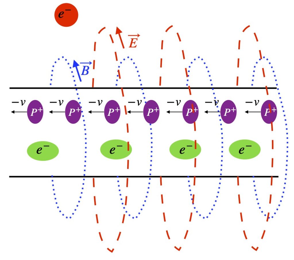
Figure 8.1 will help illustrate the answer. When special relativity is being considered, things are the same as in figure 1.3 in the frame of reference. We would expect some length contraction in the green electrons in relative motion and it doesn’t look like there is any in the diagram. However, we assume that if the electrons were at rest with respect to the frame of reference, they would have been bigger. In fact, when we look at frame in the setting of special relativity, we see this.
In frame , our frame of reference is moving with the same rightward velocity as the red test electron and green electrons in the wire. Thus, these electrons appear to be at rest in this frame. Accordingly, the electrons in the wire are greater in diameter than they are in frame (i.e., they return to their normal diameter). However, in frame , the protons have relative velocity to the left. Because they’re moving relative to an observer in this frame, to such an observer, their diameter is smaller than in frame .
The effect of the larger diameter in the green electrons is that they become more spread out, decreasing their density, and thus, decreasing their charge density. On the other hand, the smaller diameter of the moving protons causes them to crowd together more. This crowding increases their charge density. The net effect is to produce a positive charge in the segment of wire we’re considering. And associated with this new positive charge density is a new electric field. This causes an attractive force on the test electron, pulling the test electron toward the wire. Note that the moving protons still cause a magnetic field. However, because the test electron is not moving in this frame of reference, it experiences no magnetic force.
The question then becomes, Does the downward force on the test electron caused by the electric field in frame equal the downward force on the test electron caused by the magnetic field in ? Or put another way, is the path of the test electron the same in both frames? In fact, the answer to both of these questions is “yes.” The math involved in proving this is somewhat tedious. However, for those interested in seeing this proof, click .
We’ve considered simple cases in which the test electron is either completely at rest with respect to electrons in the wire or moving exactly at the velocity of the wire’s electrons, exactly perpendicular to any magnetic field generated by the wire. In other frames of reference where these simple conditions are not met, a more complicated combination of electric and magnetic fields exert force on the test electron. Indeed, a more complex mathematical object, the electromagnetic field tensor, is needed to capture this more complex physical behavior. I won’t address this issue here but I hope, in the future, to create a separate page on electromagnetism that does discuss this subject.
IX. Experimental Confirmation
The experimental evidence confirming the predictions of special relativity is overwhelming. No experiment has ever been performed which contradicts the predictions of special relativity. References that summarize some of the evidence supporting special relativity are:
Tom Roberts and Siegmar Schleif, What is the experimental basis of Special Relativity?, 2007, accessed 13 January 2024.
Wikipedia, Tests of special relativity, accessed 13 January, 2024.
Three of the classic experiments confirming the predictions of special relativity are described below.
IX.1 Alväger et al (Speed of Light is Always c)
In 1964, T. Alväger et al, working at CERN, published an often-cited paper that proved the speed of light is always measured as c (= 2.99792458 x 1010 cm/s). Figure 9.1.1. is a schematic of the experimental setup. The actual details of the experiment are more complicated but figure 9.1.1 conveys the general idea.
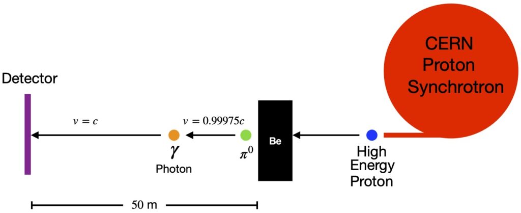
Protons were accelerated to high energy and used to bombard a beryllium plate, producing pi mesons. The resulting pi mesons (made up of a quark and an antiquark) had energies of > 6 GeV and traveled at a speed of v = 0.99975 c. The produced particles can be positively charged, negatively charged or electrically neutral. Magnets were used to sweep away all the charged varieties (not shown) leaving only neutral pi mesons (π0). These particles decay quickly into high energy photons in the gamma range. (The average lifetime of π0 particles is ~8.5×10⁻¹⁷ seconds.) The photons are detected on a screen. Since 1) the distance between the beryllium target and the detector screen and 2) the time elapsed between beryllium target bombardment and photon detection, both were known, the speed of the photons could be calculated.
Nonrelativistic physics predicted that the speed of the photons should have been 0.99975 c + 1c = 1.99975 c. Special relativity predicted that the observed photon speed should have been c. To see this calculation, click .
![\[ u=\frac{u^{\prime}+v}{1 + \displaystyle \frac{u^{\prime}v}{c^2}} \]](https://www.samartigliere.com/wp-content/ql-cache/quicklatex.com-a194ef0f1359227ac71e9644ba2f6a4a_l3.png "Rendered by QuickLaTeX.com")
 is the expected speed of the photons measured in the experiment
  is the speed of the photons in a vacuum = c
So what did Alväger et al find? They measured the velocity of the photons as 2.9977 ± 0.0004 × 1010 cm/s which is well within limits of error of the known value of c.
IX.2 Muons (Time Dilation/Length Contraction)
A muon is a fundamental particle similar to an electron with an electric charge of -1 and a spin of 1/2 but with a much greater mass. Muons are formed when high-energy protons and atomic nuclei that move through space at near the speed of light collide with particles in our upper atmosphere, about 10,000 meters above the Earth. They move at a velocity of 0.98c. Therefore, one would expect that it would take 34 x 10-6 seconds to travel from a height of 10,000 m to the Earth’s surface:

where
 is the time it takes to get from 10,000 m in the sky to the ground
 is meters
is seconds
Muons are short-lived. Their half-life, as measured in the laboratory, is 1.56 x 10⁻⁶ seconds. That means that, after 1.56 x 10⁻⁶ s, one-half of the muons decay (into an electron and two kinds of neutrinos), leaving one-half of the original number of muons intact. So, if we start with 1000 muons, after 1.56 x 10⁻⁶ s, 500 muons will have decayed and we’d be left with 500 muons. After another 1.56 x 10⁻⁶ s, half of 500 (i.e. 250) muons will decay and 250 muons will remain. After another 1.56 x 10⁻⁶ s, half of 250 (i.e. 125) muons will decay and 125 muons will be left, and so on. We can come up with an equation for this behavior as follows:

We can generalize this relationship as:
![\[ N = N_0(\frac12)^h = N_0(2)^{-h} \quad \text{(9.2.3)}\]](https://www.samartigliere.com/wp-content/ql-cache/quicklatex.com-f7ff7a5cc5e8b1d02e2e6af59f67a6d8_l3.png "Rendered by QuickLaTeX.com")
where  is the number of half-lives that have elapsed.
We ultimately want to know how many muons make it to the ground. We’ll calculate this number under 3 conditions:
- Using non-relativistic physics, from an earth-bound observer’s frame of reference
- Using special relativity, from an earth-bound observer’s frame of reference
- Using special relativity, from a frame of reference of an observer moving with a muon
Non-Relativistic, Earth Frame of Reference
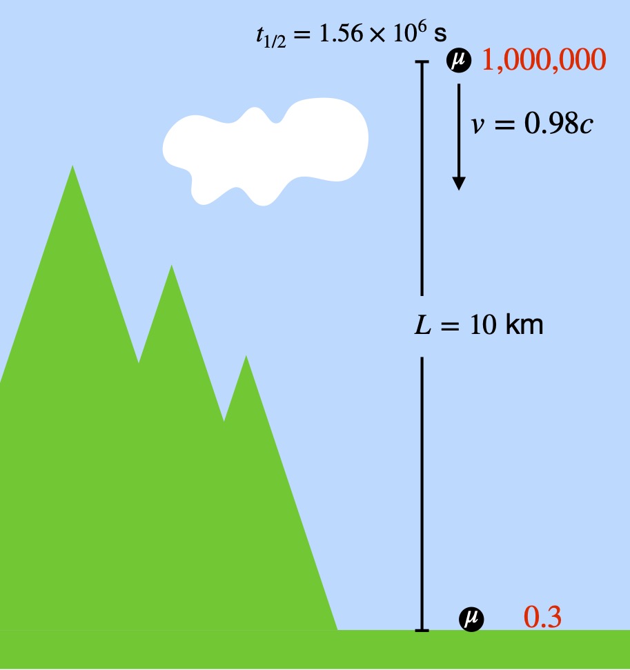
We know the time it takes to get from 10,000 m in the sky to the ground. We also know how long the half-life of a muon is (as measured in a laboratory, on the ground). Therefore, we can figure out how many half-lives it takes for a muon to hit the ground:

Thus, if we start with 1,000,000 muons, then after 21.8 half-lives:

From these calculations, we’d expect to detect only about 0.3 out of every 1 million (or about 1 out of every 3.7 million) muons produced.
Relativistic, Earth Frame of Reference
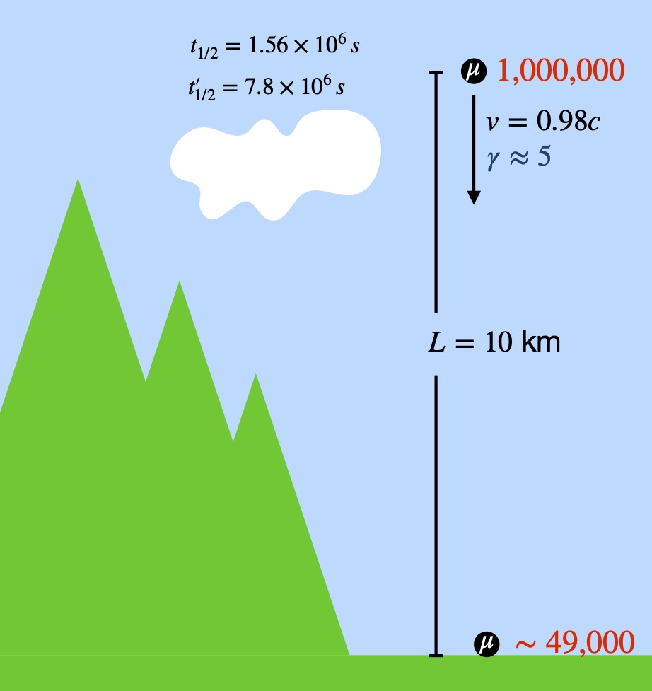
Since the muons are moving relative to an observer on the Earth, the observer on the Earth sees the “internal clocks” of the muons as running slower than his clock. Thus, the time before a muon decays (which determines the muons half-life) should take longer. Specifically:

Recall, it takes  for a muon to traverse the 10,000 m from the atmosphere to the ground. Therefore, the number of half-lives elapsed during this trip is:
![\[ \frac{34 \times 10^{-6} \text{ s}}{\sim 7.8 \times 10^{-6} \, \displaystyle \frac{\text {s}}{\text{half-life}}} = 4.36 \text{ half-lives} \quad \text{(9.2.7)}\]](https://www.samartigliere.com/wp-content/ql-cache/quicklatex.com-38ba4ee9c1493567842606efdadf9a64_l3.png "Rendered by QuickLaTeX.com")
Thus, the number of muons that reach the ground per million when time dilation is considered is:

Relativistic, Muon Frame of Reference
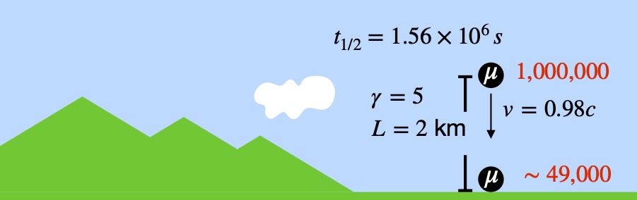
In the frame of reference of an observer traveling with the muons, the muons are at rest and the Earth is rushing toward them at 0.98c. Since we’re working under the assumptions of special relativity, the length that the earth must travel to reach the muon, from the muon’s point of view, is length-contracted. In particular:

The time it takes for the Earth to get to the muons is:

The number of half-lives this time represents is:
![\[ \frac{6.8 \times 10^{-6} \text{ s}}{1.56 \times 10^{-6} \, \displaystyle \frac{\text {s}}{\text{half-life}}} \approx 4.38 \text{ half-lives} \quad \text{(9.2.11)}\]](https://www.samartigliere.com/wp-content/ql-cache/quicklatex.com-4fe626b09f1f78df5624638800d7bb31_l3.png "Rendered by QuickLaTeX.com")
The number of muons that survive when the Earth gets to them, then, is:

So have experiments been done to test whether muons behave according to the non-relativistic or relativistic paradigm? They have. The first of these, published in 1941, is described below.
Rossi and Hall Experiment
In 1941, Bruno Rossi and David B. Hall measured the number of muons detected 1) on the top of Mount Washington in New Hampshire, a peak that’s 2000 m high, and 2) on the ground below. They detected 570 muons per hr on the mountain top. Using calculations identical to those presented above, they predicted that they would measure approximately 25 muons per hour on the ground when they used the non-relativistic methods. Using special relativity, they predicted that they would detect about 400 muons per hour on the ground. What did they find? Results agreed with special relativity. Numerous experiments similar to this have been performed since. All agree with special relativity.
IX.3 Hafele and Keating (Twin Paradox)
In a 1971 paper, J.C. Hafele and R. E. Keating, Science 177, 166 (1972), describe their experiment in which they loaded 4 ultra-accurate cesium atomic clocks onto 2 planes, flew them around the world in opposite directions, then compared the clocks’ readings to 4 cesium clock remaining on the Earth, at the United States Naval Observatory. One of the planes flew eastward (Plane A, red in figure 9.3.1), with the direction of the Earth’s rotation. The other flew westward (Plane B, blue in figure 9.3.1), against the Earth’s rotational motion. The speed of the Earth’s rotation is 463 m/s. The eastbound plane speed was 685 m/s. The westbound plane speed was 241 m/s.
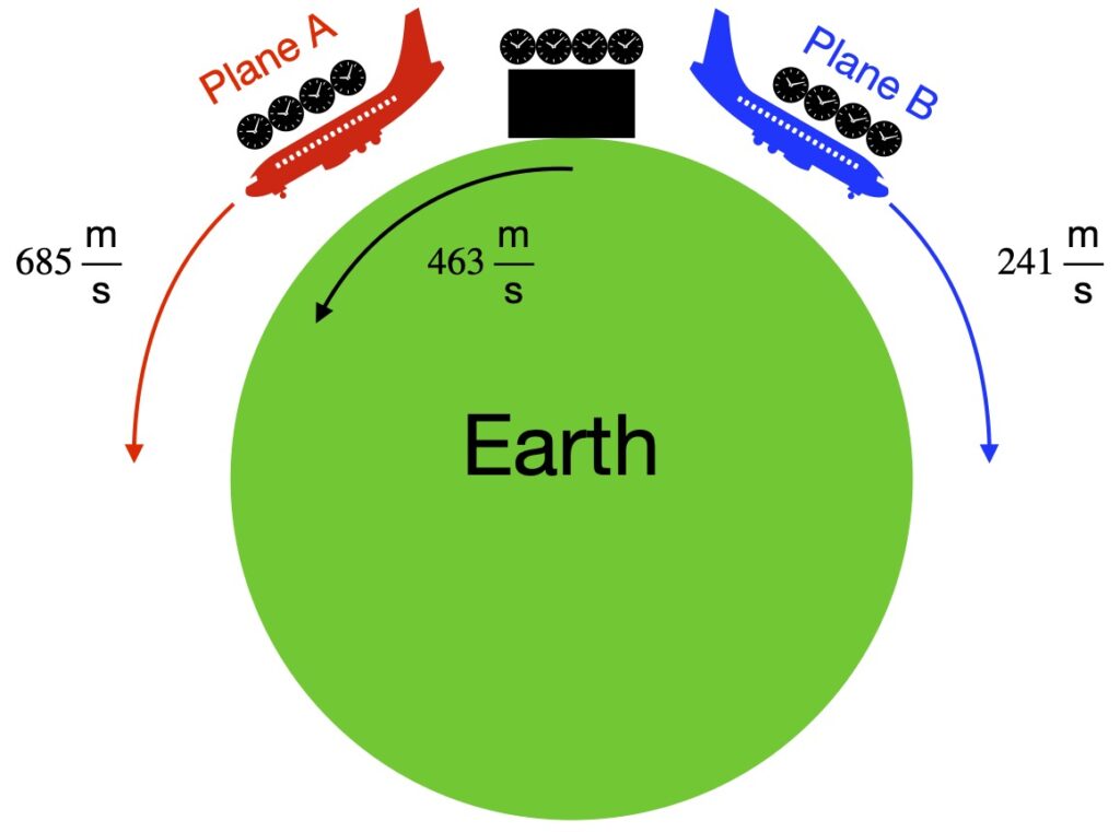
Due to time dilation, it was expected that because
- Plane A flew at higher velocity relative to the ground clocks, its clocks would tick slower than the ground clocks and thus would read an earlier time than the ground clocks
- Plane B flew at lower velocity relative to the ground clocks, its clocks would tick faster than the ground clocks and thus would read a later time than the ground clocks
However, another factor had to be considered: time dilation due to general relativity. The motion of the planes was further away from the Earth’s center than the clocks on the Earth’s surface. Therefore, clocks on the plane were expected to tick faster than the clocks on the Earth’s surface. This factor had to be adjusted for when examining results.
Results of the experiment are given in Table 9.3.1:
| Time Difference (compared with earthbound clocks) in nanoseconds | |||
| Eastward (Plane A) | Westward (Plane B) | ||
| Predicted | Gravitational | 144 +/- 14 | 179 +/- 18 |
| Kinematic | -184 +/-18 | 96 +/- 10 | |
| Net effect | -40 +/- 23 | 275 +/- 21 | |
| Observed | -59 +/- 10 | 273 +/- 21 | |
In the table, a positive time difference means the clocks ticked faster than the clocks on Earth, and therefore, would show a later time than the earthbound clocks after the trip. A negative time difference means the clocks ticked slower than the clocks on Earth, and thus, would show an earlier time than the earthbound clocks after the trip. As noted above, it was calculated that the Earth’s gravity should make the clocks on both planes tick slower than earthbound clocks. Therefore, the effect due to gravity on both planes’ clocks was positive. The term”kinematic” in the table refers to special relativity effects. Within limits of error, the observed effects due to special relativity (i.e., the net effects) agreed with predictions (i.e., the net effects).
Thus, this experiment proved 1) that the time dilation predicted by special relativity is real and 2) that an object making a round trip will come back to an initially same-aged object that remained at relative rest and will be younger than the stationary object (i.e., it proved that the twin paradox is not a paradox).
Numerous additional experiments have since corroborated these results. In fact, these results are confirmed everyday as GPS devices depend on exactly these effects to function properly.