Introduction
Lagrangian mechanics is a formulation of classical physics that is an alternative to Newtonian Mechanics. In Lagrangian mechanics, given an entity, the Lagrangian,  , if one minimizes the trajectory of a particle through phase space (a plot of position versus time), then the equation that describes this trajectory can by used to derive Newton’s equations of motion. One of the advantages of the Lagrangian system is that the equations of classical physics all stem from a single expression – the Lagrangian. Another important feature of Lagrangian mechanics is that its methodology can be adapted to advanced theories in physics such as relativity, quantum mechanics and quantum field theory.
In the following section, we will derive the Euler-Lagrange equation, the key equation in this formulation.
Derivation of Euler-Lagrange equation
Adapted from Khan Faculty
Particles in nature follow a specific trajectory through space which translated to a specific trajectory on a phase space diagram (which, as mentioned above, is a plot of position versus time). If we specify two points in phase space,  and
and  , there are an infinite number of possible paths that a particle can take in traveling from
  to
to  .
.
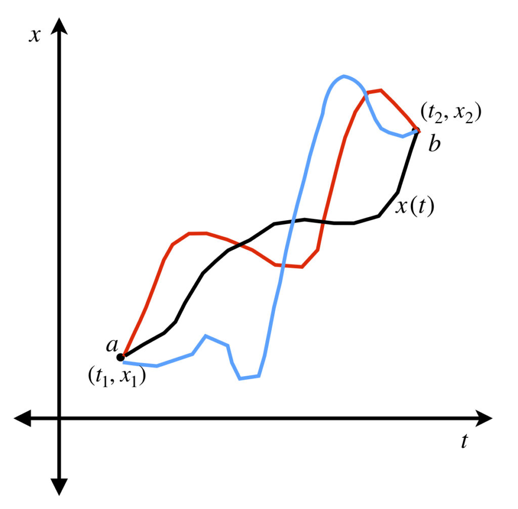
Yet , given a specific set of initial conditions (position and velocity) and an environment of potential energy (which may vary with time and creates forces), the particle takes only one of these paths. The solution of the Euler-Lagrange equation elucidates the laws that determine this path. Here is its derivation:
The problem we want to solve can be stated as follows:
Find  such that the functional

is stationary given the boundary conditions  and
and  .
.
Here are two important points to clarify before we really get into it:
First, what is a functional? A functional is simply a function of a function. In the case we are developing the functional with which we will be concerned is the Lagrangian, which is a function of position,  , and velocity,
  , which themselves are functions.
Second, what does it mean to be stationary?
Well, in single or multivariable calculus, it means that the value of a function is 1) a local maximum (i.e., its value rises to a local maximum value then decreases again) 2) a local minimum (i.e., its value decreases to a local minimum then increases again) or 3) is a saddle point (i.e., for a function of greater than 2 dimensions, is at a minimum in one direction and is at a maximum in another direction). Why is it called stationary? Because at every one of these 3 types of points, the slope of the function (which is its derivative) has to go from positive to negative or negative to positive. To do this, it has to go through a point where the value of its slope (=derivative) is zero. That point is the maximum, minimum or saddle point.
It has a slightly different (though kind-of related) meaning as it applies to the calculus of variations (which is what we’ll be doing in this derivation). In a calculus of variations problem, the goal is to find the equation of the shortest pathway between two points. As we shall see, the way that this is done is to find a curve where the sum of the deviations from the optimal path is zero. This condition of zero deviation from the optimal pathway is what it means for a functional to be stationary.
Now, on to the meat of the derivation.
Let’s assume that a function makes  stationary and satisfies the above boundary conditions ( and ).
Introduce a function,  , which we’ll see in a minute, will, create a deviation from in functionals. Since the functionals have to end on the same endpoints as ,
  and
and  (i.e., the deviation of the functional from the endpoints is zero).
Define a series of functionals (which describe an infinite number of curves),  . These functionals satisfy the same boundary conditions as . Note also that all of the functions we’ve defined here are continuous functions that have a second derivative that’s defined.
What we want to do is find the particular  that makes
  stationary. We deal with
  because
  is the only thing that changes the value of of . Why?
- First,
 doesn’t change because it’s an independent variable which gets “integrated out” of the expression for .
 - Second, . Both and are “fixed” functions along .
- Therefore, the only thing that will change the value of , and thus 1) create different curves that we can check to see if that curve is the stationary curve, and 2) in turn, change the value of , is .
To make stationary, what we have to do is set its derivative equal to zero: 
If  that means that

We apply the chain rule to the derivative inside the integral sign:
![\int\limits_{t_1}^{t_2}\left[ \frac{\partial L}{\partial \bar{x}}\frac{\partial\bar{x}}{\partial \epsilon} + \frac{\partial L}{\partial\bar{x}^\prime}\frac{\partial\bar{x}^\prime}{\partial\epsilon} \right]dt = 0](https://www.samartigliere.com/wp-content/ql-cache/quicklatex.com-8ee3e4e76a1568268b1f9190a7f0cc67_l3.png "Rendered by QuickLaTeX.com")
Next we need to find the derivatives of  and
and  :
:

Substituting the values for  and
and  we just calculated:
![\int\limits_{t_1}^{t_2}\left[ \frac{\partial L}{\partial \bar{x}}\eta + \frac{\partial L}{\partial\bar{x}^\prime}\eta^\prime \right]dt = 0](https://www.samartigliere.com/wp-content/ql-cache/quicklatex.com-8a3605ca331a6d099fa2b9ff4dd085b3_l3.png "Rendered by QuickLaTeX.com")
We can apply integration by parts to the term  . In integration by parts:

Let  and
and  . Then

But  . Thus,
  . From our definition of above,
  . Therefore,
  . That leaves us with

Substituting in the last expression, we get:
![\int\limits_{t_1}^{t_2}\left[ \frac{\partial L}{\partial \bar{x}}\eta - \eta \frac{d}{dt}\frac{\partial L}{\partial \bar{x}^\prime} \right]dt = 0](https://www.samartigliere.com/wp-content/ql-cache/quicklatex.com-3740d973997b887eb3dae1d90d803146_l3.png "Rendered by QuickLaTeX.com")
Factor out  :
:
![\int\limits_{t_1}^{t_2}\left[ \frac{\partial L}{\partial \bar{x}} - \frac{d}{dt}\frac{\partial L}{\partial \bar{x}^\prime} \right]\eta dt = 0](https://www.samartigliere.com/wp-content/ql-cache/quicklatex.com-0533ef883b2765fd40a024bf32d3740f_l3.png "Rendered by QuickLaTeX.com")
When 

and
 .
.
Therefore, the above integral becomes:
![\int\limits_{t_1}^{t_2}\left[ \frac{\partial L}{\partial x} - \frac{d}{dt}\frac{\partial L}{\partial x^\prime} \right]\eta dt = 0](https://www.samartigliere.com/wp-content/ql-cache/quicklatex.com-fd467e416eeac1ab737cd92a7c7b5116_l3.png "Rendered by QuickLaTeX.com")
So we’ve met our criteria for making stationary:
 and
and
There’s just one thing left to do.
In order for the above integral to equal zero, the quantity inside the integral has to equal zero. That quantity is the product of two entities, ![[\cdots]\eta](https://www.samartigliere.com/wp-content/ql-cache/quicklatex.com-bd53c550669969e8359cc11b6fbe5808_l3.png "Rendered by QuickLaTeX.com") and this product must equal zero. But is a nonzero function. Therefore, in order for the product to be zero, the stuff inside the brackets has to equal zero:
and this product must equal zero. But is a nonzero function. Therefore, in order for the product to be zero, the stuff inside the brackets has to equal zero:
(1) 
This equation is the Euler-Lagrange equation.
Application of the Euler-Lagrange equation to physics
We derived the following equation and identified it as the Euler-Lagrange equation:

Furthermore, we’ve said that this equation is derived from the fact that an entity, does not change.
As it applies to physics:
- is called the action.
 is called the Lagrangian of a system.
 is referred to as the principle of least action, or more appropriately, the principle of stationary action.
As stated at the outset of this article, Newtonian mechanics can be derived from this principle. The specific example we’ll use to illustrate this is derivation of Newton’s second law of motion from the Euler-Lagrange equation.
In classical mechanics, for a particle moving through a potential energy field, the Lagrangian, , equals the kinetic energy of the particle minus the potential energy affecting that particle:
 where
where
 = mass of the particle
 =
=  =
=  = velocity of the particle
 = potential energy, which is a function position,
In these equations, we’re using to represent the time derivative of instead of  or because this is the convention used for the Euler-Lagrange equation in most textbooks and papers. Also, if we were considering a particle moving in 3-dimensional space, we would have to use partial derivatives to differentiate and . However, in this example, we’ll considering a particle moving in only one direction of space – the direction. Thus, we can use regular derivatives when differentiating and . We still have to take partial derivatives when differentiating though because is a function of two variables.

The only term that depends on is the potential energy term,  . Therefore,

The only term that depends on is the kinetic energy term,  . Therefore,

That means that

which, of course, is Newton’s second law of motion.
The Euler-Lagrange equation is frequently written:

In this equation,  and
and  are called generalized coordinates. They could be any kind of coordinates (e.g., polar, cylindrical, spherical, etc.). represents spatial position and represents velocity based on such coordinates. The
  subscripts specify individual particles. To describe an entire ensemble of particles, we would need one equation for each particle.
Note that, although the equations of motion for some physical systems may be quite complicated, the principle of stationary action can be applied to all of them, including systems that require such advanced descriptions as general relativity, quantum mechanics, quantum field theory and string theory . For such varied systems, the Lagrangian may take many different forms. How are these Lagrangians determined? Sometimes from some previous knowledge; sometimes from an educated guess based on some physical theory; sometimes from results of experiments – in short, by whatever method works.
The simple Lagrangian that describes particles moving through a potential energy field that we worked with above is a case in point. As far as I can tell, there is no specific intuition to explain the form of this expression except that it works.
There is some intuition, however, to explain why the stationary action principle works. This intuition stems from quantum mechanics and is well-explained in an article from UVA. The argument goes something like this:
According to quantum mechanics, particles aren’t really particles. They’re waves. At least, the probability of measuring them in a given location is described as a wave. Waves that are near each other have wavefronts that are nearly in phase and interfere with each other constructively. On the other hand, wavefronts that are farther away tend to be out of phase and interfere with each other destructively. The locations where the waves interfere constructively are the locations where the light (or other “particle”) is most likely to be found. These locations constitute the path described by the stationary action principle.