Bell’s Inequality 3

Introduction
Experimental Set-up
Predictions: Classic vs. Quantum
- Classical Predictions
- Quantum Predictions
Results
Conclusion
References

Introduction

In the first installment in this series,¹ we provided an introduction to Bell’s inequality including an intuitive demonstration about how it works. In the second installment,² we discussed Bell’s 1966 paper and derived his original inequality that he presented in that paper. However, while that inequality provided a potential way to test whether a classical local hidden variables theory or quantum mechanics represents reality, it does not offer evidence regarding which of these possibilities is true. It was several years before such experiments were carried out. One of the most often-cited of these papers is the second of three written by Alain Aspect in the 1980s, specifically, the one published in 1982.^3, ⁴ This webpage gives a step-by-step explanation of Aspect’s 1982 paper in an attempt to make it understandable to non-experts. However, to achieve such understanding, it is suggested that parts I and II of this series be read first.

Experimental Set-up

The experimental set-up used by Aspect differs from the thought experiment outlined in Bell’s original paper. First, Aspect measures polarization of entangled photons instead of the entangled electrons considered in Bell’s paper. Second, Aspect employs a two-channel polarizer and two detection screens at each measurement site. Don’t ask me how a two-channel polarizer works; I don’t know. However, what it does is split an entangled photon into two photons that are polarized at different angles, sending each off to a different detector at the same measurement site. Thus, four measurements can be made for each run of the experiment. The importance of this will become evident shortly.

An overview of the experimental setup is given in the following diagram:

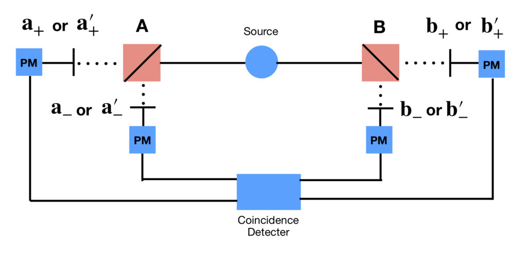
This is how it all works. Lasers are shot at a beam of calcium-40 atoms and entangled linearly polarized photons are shot off at opposite directions, one toward A and one toward B. A more detailed discussion of photon polarization can be found elsewhere on this website.⁵ Here is a review of what needs to be known for our discussion here:

Linear polarization of a photon refers to the angle at which the electromagnetic wave associated with this photon propagates in space.
Polarization filters are devices that are used to measure photon polarization angle. They are set at specific angles.
If the angle at which an approaching photon is polarized matches the angle at which the filter is set, then the photon will pass through the filter, 100% of the time.
If the angle at which an approaching photon is polarized is at an angle that is orthogonal (i.e., perpendicular; at $90^\circ$ ) to the angle at which the polarization filter is set, then the photon will not pass through the filter, 100% of the time.
If the angle of polarization of an approaching photon differs from the angle at which the polarization filter is set by any other amount, then the photon will pass through the filter some but not all of the time.
The entangled photons in Aspect’s experiment always both exhibit the same angle of polarization when they are measured.⁶

Here are some additional facts regarding Aspect’s experimental setup:

The filter at A is set to one of two angles: $a=0^\circ$ or $a^\prime=45^\circ$ . The filter at B is set at either $b=22.5^\circ$ or $b^\prime=67.5^\circ$ .
Choice of filter angle at A and B are independent and random.
Because a dual channel polarizer is used, a photon that is parallel to a polarization filter is labelled +1 and is passed to a photomultiplier which sends an electrical signal to a coincidence detector. On the other hand, a photon whose polarization angle is oriented perpendicular to a filter is labelled -1 and is passed to a different photomultiplier which sends an electrical signal to a different part of the coincidence detector.
Also because a dual channel polarizer is used, one photon from the A side and one photon from the B side will reach the coincidence detector for each pair that is emitted (at least theoretically). This is an advantage over experiments that use single channel polarizers since, with single channel polarizers, photons polarized perpendicular to the filter will not reach the coincidence detector. If this occurs, one cannot be sure whether this is because of true perpendicular polarization or equipment failure.
Once signals instigated by photons from A (either +1 or -1) and B (either +1 or -1) reach the coincidence detector, their values are multiplied together, yielding, again, either +1 or -1.
These products are tabulated and used to calculate an expectation value (=average or mean) for each of the possible filter angle configurations: $(a,b)$ , $(a,b^\prime)$ , $(a^\prime,b)$ , $(a^\prime,b^\prime)$ .
The four expectations values are then combined to produce a statistic, $S$ .
The classical local hidden variable theory advocated by Einstein et al and quantum mechanics predict different values for $S$ . This is how the experiment determines which theory is correct.

Predictions: Classical vs. Quantum

So we said that Aspect’s experiment is supposed to tell which theory of physics is correct, a classic local hidden variables theory or quantum mechanics. And it does this by seeing with the predictions of which of these theories experimental results agree. So what are the predictions of each of these theories?

Classical Predictions

Let’s start with the predictions of the classical theory. Recall that, according to such a theory, there is(are) some hidden variable(s) that, in essence, render some program to the entangled photons, telling them how they should behave in every circumstance. Thus, it is these hidden variables combined with the angle of depolarization filter settings that determine the results of an experiment.

One might think, given all the effort that was spent in a previous article on Bell’s original inequality, that it might be this inequality that forms the basis for Aspect’s experiment. It turns out, however, that it is another form of Bell’s inequality, the so-called CHSH inequality named after its inventors, John Clauser, Michael Horne, Abner Shimony and R. A. Holt, that Aspect’s paper uses. As will become evident shortly, this is because dual channel polarization filters are used in Aspect’s experiment. The CHSH inequality is a generalization of the original Bell’s inequality; the original Bell’s inequality is just a special case of the CHSH version. As mentioned above, the CHSH inequality makes use of a quantity called $S$ . It takes the following form:

$2 \leq S \geq 2$

where

$S=E(a,b)-E(a,b^\prime)+E(a^\prime,b)+E(a^\prime,b^\prime)$

and the $E's$ are expectation values that are found when the polarizers at A and B are set at the angles indicated in the parentheses that appear after the $E's$ . Recall from the discussion in Bell’s Inequality 2 that an expectation value is an average value or mean value of a given quantity. In Aspect’s experiment, the value of the measurement at A (either + or – 1) and the simultaneous measurement at B (either + or – 1) are multiplied together. The product of the measurements of A and B is also +1 or -1; +1 if the sign of the measurements at both A and B are the same (i.e., both + or both -) and -1 if the sign of the measurements at A and B are different. What the expectation value, $E$ , represents is the average of the products of these measurements that are obtained on each run of the experiment. This can be expressed mathematically as follows:

Let

$A=A(a,\lambda)$ = the measurement obtained at A, determined by the angle of polarization, $a$ , and some hidden variable, $\lambda=\pm1$
$A^\prime=A^\prime(a^\prime,\lambda)$ = the measurement obtained at A, determined by the angle of polarization, $a^\prime$ , and some hidden variable, $\lambda=\pm1$
$B=B(b,\lambda)$ = the measurement obtained at B, determined by the angle of polarization, $b$ , and some hidden variable, $\lambda=\pm1$
$B^\prime=B^\prime(b^\prime,\lambda)$ = the measurement obtained at B, determined by the angle of polarization, $b^\prime$ , and some hidden variable, $\lambda=\pm1$

From the discussion on expectation values in Bell’s Inequality 2,

$E(a,b)=\int AB \rho(\lambda)d\lambda$
$E(a,b^\prime)=\int AB^\prime \rho(\lambda)d\lambda$
$E(a^\prime,b)=\int {A^\prime}{B} \rho(\lambda)d\lambda$
$E(a^\prime,b^\prime)=\int{A^\prime}{B^\prime}\rho(\lambda)d\lambda$

Because, as stated above, $S=E(a,b)-E(a,b^\prime)+E(a^\prime,b)+E(a^\prime,b^\prime)$ it follows that

$\begin{array}{rcl}S &=& \int AB \rho(\lambda)d\lambda-\int AB^\prime \rho(\lambda)d\lambda+\int {A^\prime}{B} \rho(\lambda)d\lambda+\int{A^\prime}{B^\prime}\rho(\lambda)d\lambda\\ &=& \int\left(AB+{A}{B^\prime} + {A^\prime}{B}+{A^\prime}{B^\prime}\right)\rho(\lambda)d\lambda\\ &=& \int A(B-B^\prime) + A(B+B^\prime)\end{array}$

The following table shows what happens to the expressions that make up the right side of the last equation listed above (and therefore, $S$ ) if we put in the most extreme (i.e. highest magnitude) values that $A$ , $B$ and $B^\prime$ can take (i.e., +1 or – 1):

$B$	$B^\prime$	$B-B^\prime$	$B+B^\prime$	$A(B-B^\prime)$	$A(B+B^\prime)$
+1	+1	0	2	0	$\pm2$
+1	-1	2	0	$\pm2$	0
-1	+1	-2	0	$\pm2$	0
-1	-1	0	-2	0	$\pm2$

From the table, one can see that the minimum and maximum values that the sum of $A(B-B^\prime)$ and $A(B+B^\prime)$ (and thus $S$ ) can have are -2 and +2, respectively. That means that

$2 \leq S \geq 2$ , as stated above.

Quantum Predictions

Next we need to see what quantum physics predicts for the value of $S$ . Let’s start by calculating an expression for the quantum mechanical prediction of the expectation values. Let’s take $E(a,b)$ as an example. For the experimental circumstances used in Aspect’s paper (i.e., one entangled photon at A measured at angle $a$ ; its entangled partner, evaluated at B, measured at angle $b$ ) we have:

$E(a,b)= \frac{P_{++}(a,b)\,+\,P_{--}(a,b)\,-\,P_{+-}(a,b)\,-\,P_{++}(a,b)}{P_{++}(a,b)\,+\,P_{--}(a,b)\,+\,P_{+-}(a,b)\,+\,P_{++}(a,b)}\quad \text{where}$

$\begin{array}{rcl}P_{++}(a,b) &=& \text{the probability of the product of measurements at both \textbf{A} and \textbf{B} being} \, +1 \\ P_{--}(a,b) &=& \text{the probability of the product of measurements at both \textbf{A} and \textbf{B} being} \, -1 \\ P_{+-}(a,b) &=& \text{the probability of the product of measurements at \textbf{A} = +1 and \textbf{B} = -1}\\ P_{-+}(a,b) &=& \text{the probability of the product of measurements at \textbf{A} = -1 and \textbf{B} = +1} \end{array}$

According to the edicts of quantum mechanics, when a photon approaches a polarization filter, it is in a superimposition of states in which it is polarized at all angles simultaneously. When it hits the filter, it becomes polarized, with an equal probability, either parallel or orthogonal (=perpendicular) to that angle at which the filter is set. As previously described, because a dual channel polarization filter is in use, the photon is split, the parallel photon passing to the +1 detector and the orthogonal photon passing to the -1 detector. From this, we have,

$\begin{array}{rcl}P_+(a) &=& \text{the probability that a photon measured at \textbf{A} at angle }a\, \text{is measured as} +1 = 1/2\\ P_-(a) &=& \text{the probability that a photon measured at \textbf{A} at angle }a\, \text{is measured as} -1 = 1/2\\ P_+(b) &=& \text{the probability that a photon measured at \textbf{B} at angle }b\, \text{is measured as} +1 = 1/2\\ P_-(b) &=& \text{the probability that a photon measured at \textbf{B} at angle }b\, \text{is measured as} -1 = 1/2\end{array}$

The next thing we have to figure out is: once a photon passes through a filter, say at A, what is the probability its detector output, +1 or -1, will agree with its entangled partner at B?

The following diagram will help us do this:

In the diagram, the black arrowed line labeled $a$ or $a^\prime$ indicates that an entangled photon is measured at angle $a$ or $a^\prime$ at A, depicted here in the vertical direction, a direction we’ll consider to be at $0^\circ$ . In contrast, its entangled partner is measured at B, at angle $b$ or $b^\prime$ , which differs from $a$ or $a^\prime$ by an angle $\theta$ . Since the photons are entangled, their angles of polarization have to be the same. Say the photon at B is measured as +1. That means that, with 100% probability, its angle of polarization is at the angle of measurement, $b$ or $b^\prime$ . What, then, is the probability that its entangled partner will be measured as +1 at A? According to quantum mechanics, as the entangled partner approaches A, it is polarized at the same angle as that in which its entangled partner got measured, $b$ or $b^\prime$ . It is in a superimposition of states expressed in the basis in which it is about to be measured (i.e., parallel = $0^\circ$ , orthogonal = $90^\circ$ ). Some of its polarization is parallel to (overlaps) the direction in which it will be measured (i.e., $0^\circ$ ) and some has no overlap with (is orthogonal to) the direction of measurement (in this case, that orthogonal direction would be $90^\circ$ ). In quantum mechanics, this state of superimposition is given by probability amplitudes that are associated with each polarization direction component. The direction that would yield a +1 measurement, a measurement that agrees with the measurement at B, is the $0^\circ$ direction. As depicted in the diagram, the probability amplitude associated with that direction is given by $\cos\theta$ . Conversely, The direction that would yield a -1 measurement, a measurement that disagrees with the measurement at B, is the $90^\circ$ direction. As depicted in the diagram, the probability amplitude associated with that direction is given by $\sin\theta$ . In turn, the probability that an event will occur is given by the square of its probability amplitude. So the probability that the measurements at A and B will agree is $\cos^2\theta$ and the probability that the measurements at A and B will disagree is $\sin^2\theta$ . Note that these probabilities depend only on the difference between the angles of measurement, $\theta$ . Therefore, it doesn’t matter at what angles we measure at A and B, as long as the angle between them is the same, the probabilities will be the same.

From the above,

The probability that the measurement at A, measured in the $a$ -direction is +1 is $1/2$ . The probability that this measurement agrees with the measurement at B (=+1) measured in the $b$ direction is $\cos^2(b-a)$ which we’ll write as $\cos^2(a,b)$ . The probability that these two events occur together ( $P_+_+(a,b)$ ) is obtained by multiplying these two probabilities together. Therefore, $P_+_+(a,b)=\frac12\cos^2(a,b)$ .
The probability that the measurement at A, measured in the $a$ -direction is -1 is $1/2$ . The probability that this measurement agrees with the measurement at B (=-1) measured in the $b$ direction is $\cos^2(b-a)$ which we’ll write as $\cos^2(a,b)$ . The probability that these two events occur together ( $P_-_-(a,b)$ ) is obtained by multiplying these two probabilities together. Therefore, $P_-_-(a,b)=\frac12\cos^2(a,b)$ .
The probability that the measurement at A, measured in the $a$ -direction is +1 is $1/2$ . The probability that this measurement disagrees with the measurement at B (=-1) measured in the $b$ direction is $\sin^2(b-a)$ which we’ll write as $\sin^2(a,b)$ . The probability that these two events occur together ( $P_+_-(a,b)$ ) is obtained by multiplying these two probabilities together. Therefore, $P_+_-(a,b)=\frac12\sin^2(a,b)$ .
The probability that the measurement at A, measured in the $a$ -direction is -1 is $1/2$ . The probability that this measurement disagrees with the measurement at B (=+1) measured in the $b$ direction is $\sin^2(b-a)$ which we’ll write as $\sin^2(a,b)$ . The probability that these two events occur together ( $P_+_-(a,b)$ ) is obtained by multiplying these two probabilities together. Therefore, $P_-_+(a,b)=\frac12\sin^2(a,b)$ .

A summary of the above information is as follows:

$P_+_+(a,b)=\frac12\cos^2(a,b)$
$P_-_-(a,b)=\frac12\cos^2(a,b)$
$P_+_-(a,b)=\frac12\sin^2(a,b)$
$P_-_+(a,b)=\frac12\sin^2(a,b)$

Next we substitute these values into the expressions for the expectation value:

$\begin{array}{rcl}E_a_b&=&P_+_+(a,b)+P_-_-(a,b)+P_+_-(a,b)+P_-_+(a,b)\\ &=& \frac12\cos^2(a,b)+\frac12\cos^2(a,b)+\frac12\sin^2(a,b)+\frac12\sin^2(a,b)\\&=&\cos^2(a,b)-\sin^2(a,b) \end{array}$

But $\cos^2(a,b)-\sin^2(a,b)=\cos2(a,b)$ (proof of this can be found here)

The denominator for the expression for the expectation value, $P_+_+(a,b)+P_+_-(a,b)+P_-_+(a,b)+P_-_-(a,b)$ represents the sum of the probabilities of all of the possible combinations of $a$ and $b$ that exists. Therefore, this sum has to equal 1. Anything entity divided by one is the entity itself, so

$E_a_b=\cos2(a,b)$

Similarly,

$E_a_b^\prime=\cos2(a,b^\prime)$
$E_a^\prime_b=\cos2(a^\prime,b^\prime)$
$E_a^\prime_b^\prime=\cos2(a^\prime,b^\prime)$

We can now use these values to obtain the quantum mechanical prediction for the value of $S$ . Recall that

$S=E(a,b)-E(a,b^\prime)+E(a^\prime,b)+E(a^\prime,b^\prime)$

Inserting the quantum predictions for the expectation values into the above equation, we get

$S=\cos2(a,b)-\cos2(a,b^\prime)+\cos2(a^\prime,b^\prime)+\cos2(a^\prime,b^\prime)$

We previously noted that the polarization filter angles used in Aspect’s experiment are $a=0^\circ$ , $b=22.5^\circ$ , $a^\prime=45^\circ$ , $b^\prime=67.5^\circ$ . The reason that these angles were chosen is because they create the greatest difference between the value of $S$ predicted by a classic local hidden variable model and the value of $S$ predicted by quantum mechanics.⁴ Substituting these filter angles into the last equation yields the following:

$\begin{array}{rcl}S&=&\cos2(a,b)-\cos2(a,b^\prime)+\cos2(a^\prime,b^\prime)+\cos2(a^\prime,b^\prime)\\ &=&\cos2(22.5-0)-\cos2(67.5-0)+\cos2(0-22.5)+\cos2(67.5-45)\\ &=& \cos2(22.5)-\cos2(67.5)+\cos2(-22.5)+\cos2(22.5)\\ &=& \cos(45)-\cos(135)+\cos(-45)+\cos(45)\\ &=& 0.707-(-0.707)+0.707+0.707\\ &=& 0.707+0.707+0.707+0.707\\ &=& 2.828 \end{array}$

Like with any real experiment, equipment is not perfect. Aspect describes two sets of correction factors in his paper. One set appears to correct for inefficiencies in transmission and reception of photons. Transmission and reception rates are calculated for the parallel and perpendicular directions. The rates labeled with subscript 1 relate to transmission and reception at site A; those labeled with subscript 2 relate to transmission and reception at site B. The following values are given:

$T_1^\parallel=R_1^\perp=0.950$
$T_1^\perp=R_1^\parallel=0.007$
$T_2^\parallel=R_2^\perp=0.930$
$T_2^\perp=R_2^\parallel=0.007$

He uses these values to create the following correction factor:

$\frac{\left(T_1^\parallel-T_1^\perp \right)\left(T_2^\parallel-T_2^\perp \right)}{\left(T_1^\parallel+T_1^\perp \right)\left(T_2^\parallel+T_2^\perp \right)}=\frac{\left(0.950-0.007 \right)\left(0.930+0.007 \right)}{\left(0.950+0.007 \right)\left(0.930+0.007 \right)}=0..971$

He also applies a second correction factor, $F=0.984$ , which he says “accounts for the finite solid angles of detection.”

To be sure, a discussion of the technical limitations of the study and the corrections that account for them are critical in convincing the scientific community that the study’s results are valid. However, I am not a physicist. My background in experimental physics is especially limited. It would take an inordinate amount of time for me to dig out the details of the technical aspects of the experiment and explain them. Furthermore, the focus of this article is on the theoretical underpinnings of Bell’s Inequality not experimental details. Therefore, I will trust Dr. Aspect (who is an expert experimentalist) and show how he uses the above corrections to adjust the quantum mechanical prediction of $S$ :

$S_QM=0.984\cdot0.971\cdot2.828=2.70\pm 0.05$

Results

So what are the results of Aspect’s experiment? Do they agree with a classic hidden variables theory (i.e. $\mid S \mid \leq 2$ or quantum mechanics $S \approx 2.70$ . The experimental value of $S$ determined in the Aspect paper is

$S=2.697\pm0.015$

This value closely approximates the prediction of quantum mechanics and violates Bell’s inequality by greater than 40 standard deviations from the mean!

Conclusion

Therefore, Aspect’s results strongly support the contention that quantum mechanics is the correct description of reality.

References

1. https://www.samartigliere.com/wp-content/uploads/2018/11/Bells-Inequality-1.pdf
2. https://www.samartigliere.com/physics/quantum-mechanics/bells-inequality-2/(opens in a new tab)
3. Alain Aspect, Philippe Grangier, and Gerard Roger, “Experimental Realization of Einstein-Podolsky-Rosen-Bohm Gedankenexperiment: A New Violation of Bell’s Inequalities.” Physical Review Letters, vol. 49, no. 2, July 1982, pp. 91-94, APS physics, https://journals.aps.org/prl/pdf/10.1103/PhysRevLett.49.91
4. https://arxiv.org/pdf/quant-ph/0402001.pdf
5. Photon Polarization
6. Note that entangled photons can also be prepared such that they have polarization angles that are orthogonal (i.e., perpendicular) to each other. However, this is not the case in Aspect’s experiments.

Contents