Contents
- Introduction
- Spin
- Experimental Set-up
- Proof
- Probability Distributions
- Mathematical Interlude: The Integral
- Proof (cont’)
- Significance of Bell’s Inequality
Introduction
As alluded to in the first installment on Bell’s inequality, the debate between those who believed in local realism/local hidden variables (championed by Einstein) and quantum mechanics (championed by Bohr) raged on for several decades, beginning in the late 1920’s, seemingly without any hope for resolution. Then, in 1964, Irish physicist John Bell wrote a paper (published in 1966) outlining a method that promised to break this impasse, a paper that physicist Henry Stapp called “the most profound discovery of science.”1 A description of this paper, attempting to explain the mathematics it contains, step-by-step, so that those without a mathematical background might still understand it, is the goal of this article.
Spin
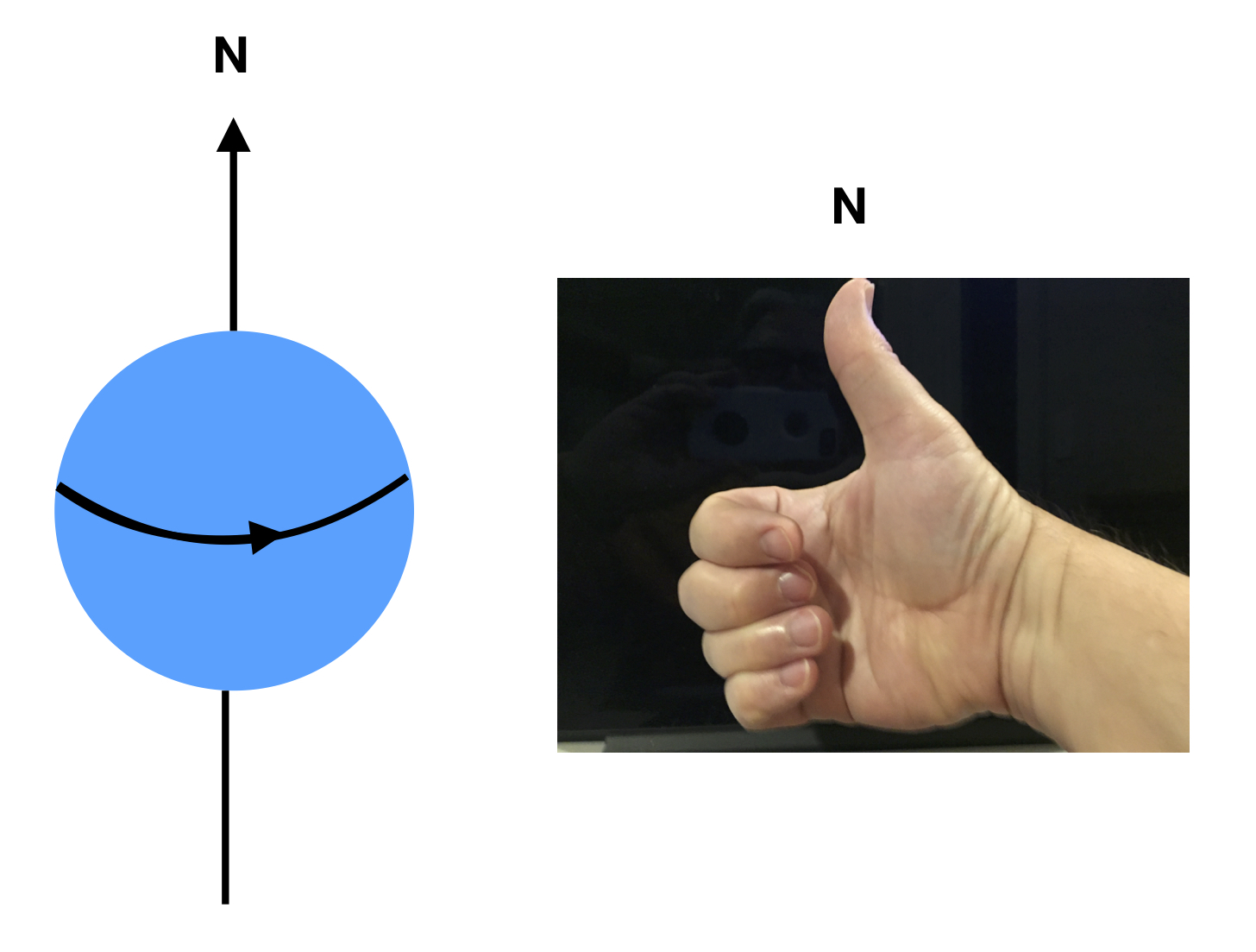
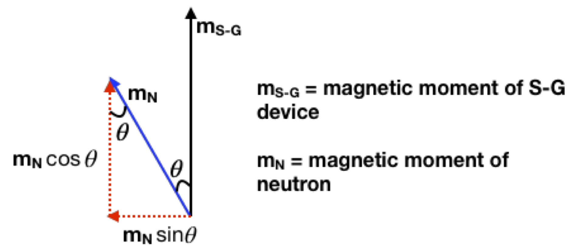
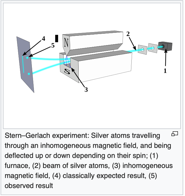
Bell considers a thought experiment designed by Bohm and Aharanov utilizing particles entangled with regards to a property called spin. Spin is a purely quantum phenomenon akin to angular momentum that, along with charge, gives particles their magnetic properties. The closest thing to it in classical mechanics is to image a spherical charged particle spinning on its axis. Such a changing electrical field will create a magnetic field that makes the particle behave in a magnetic field like a tiny bar magnet. The direction of the magnetic field (or magnetic moment) so-created can be determined by a thing called the right-hand rule: curl your fingers in the direction of a positively charged particle’s rotation and stick your thumb upward. The direction in which your thumb is pointing is the direction of the north pole of the magnet. When placed in a magnetic field, the north pole of the miniature bar magnet (or magnetic moment) will align with the magnetic field. The spin of a particle can be measured by a process called a Stern-Gerlach experiment. A Stern-Gerlach experiment employs an apparatus (we’ll call it an S-G device) consisting of a tunnel with two parallel magnetic plates, one “north-pointing” portion on one side and a “south-pointing” portion on the opposite side. In the original experiment described by Stern and Gerlach, a neutron oven shoots neutrons into the S-G device. The neutrons have a magnetic moment. This may be surprising since, even if neutrons have spin, they are electrically neutral; they have no net electrical charge. Therefore, a spinning neutron should‐at least according to classical physics‐have no magnetic moment. But it does. That’s because it’s made up of quarks which have spin and charge, and thus, magnetic moments. If you combine them, you get a net magnetic moment. At any rate, the magnetic moments of the neutrons that are shot out of the neutron oven are initially oriented in random directions. They pass through the S-G device. The magnets in the device deflect the neutrons and they are detected onto a screen at the other end of the apparatus. Since the distribution of magnetic moment directions is random, all directions should have an equal probability of being present. According to classical mechanics, the degree of deflection of any given neutron should be proportional to the magnitude of the magnetic field within the S-G device and the magnitude of the component of the magnetic moment in the direction of the magnetic field within the S-G device:
Therefore, the pattern of neutron impressions on the detection screen should be a uniform straight line. What is actually found, however, are two lumps of neutron impressions, one toward the north pole side of the S-G device and one toward the south pole side of the S-G device:
This is because the laws of quantum mechanics, not classical mechanics, govern the behavior of such subatomic particles. According to quantum mechanics, each neutron spin is in a superimposition of states that includes all possible angles-until it interacts with the S-G device and a measurement is made. At that time, because we’re measuring using a basis defined by the magnetic field in the S-G device, the neutron spin must assume one of two states: spin up (with its north pole aligned with the magnetic field of the S-G device) or spin down (with its north pole aligned against the magnetic field of the S-G device). Similar to the polarization of photons discussed in “Bell’s Inequality 1,” the probability that any given neutron will align with or against the magnetic field of the the S-G device is determined by the square of the probability amplitudes associated with the spin up and spin down neutron spin states. These, in turn, are determined by the angle between the magnetic field of the S-G device and the direction of the magnetic moment of the neutron. So the likelihood that a given neutron will be deflected upward or downward depends on the angle of its magnetic moment. However, in any given experiment, it will be deflected only in the upward or downward directions, toward the same two spots on the detection screen, never at any other angle.
Experimental set-up
The hypothetical experiment that Bell considers in his paper uses entangled electrons-spin 1/2 particles that are anti-correlated. Spin 1/2 means that they can assume only one of two possible states in the presence of an external magnetic field. Anti-correlated means that each entangled particle will always have a spin that is opposite to its partner. For example, if electron A is in the spin up state, then the spin state of its entangled partner-electron B-will, with absolute certainty, be spin down, and vice versa.
The experiment that Bell considered is as follows. An entangled electron pair is created and sent off in opposite directions, to Stern-Gerlach devices and detection screens that are set up far enough apart such that, if measured simultaneously, within limits of error, no signal sent at the speed of light could possibly get from one to the other to “tell” its entangle partner how to behave (i.e, they are what’s called “space-like separated”).
That’s simple enough. Now on to the math.
Proof
Bell begins by expressing a measurement, mathematically, as  where
where  represents the spin of an entangled electron and
  is a unit vector at some specific angle of measurement.
  and
and  then, are an entangled electron pair. Because the electrons are entangled, if
  is measured as +1, then, with 100% certainty,
  will be measured as -1, and vice versa. Bell notes that because 1) the measuring devices are far enough apart 2) the measurement are performed near simultaneously, and 3)nothing in the universe can go faster than the speed of light, this result could not have come about due to one particle influencing the other. Then, for the purposes of his discussion, he takes the viewpoint of Einstein, Podolsky and Rosen (EPR), reasoning that there must have been that some hidden variable (or collection of hidden variables), acting at the time the particles interacted, “programming” the particles to behave as they did. He calls such hidden variables(s)
  . Thus, he says, the result,
  , of measuring
  depends on
  and ; and the result,
  , of measuring
  depends on
  and . In addition, as discussed in our brief introduction, the results of any measurement, or , can only be +1 or -1 (i.e., spin up or spin down). Mathematically, this is expressed as

And as discussed above, an assumption vital to this article is that the result for particle 2 does not depend on the setting, , of the magnet for particle 1, nor on .
He goes on to make the following arguments:
If  is the probability distribution of then the expectation value (or average) of the product of the two components
  and
and  is
is

This should be equivalent to what quantum mechanics predicts will happen-the so-called expectation value (i.e., the average or mean)

Before proceeding, it may be helpful to say a few words about probability distributions and their properties.
Probability distributions
We said that is a probability distribution. A probability distribution is a plot of some entity versus its probability of occurrence. For example, say nine students take a test. A probability distribution of their scores are as follows:
| Score | Probability |
 = 60 = 60 | 1/9= 0.11 = 11.1% |
 = 70 = 70 | 2/9 = 0.22 = 22.2% |
 = 80 = 80 | 3/9 = 0.33 = 33.3% |
 = 90 = 90 | 2/9 = 0.22 = 22.2% |
 = 100 = 100 | 1/9 = 0.11 = 11.1% |
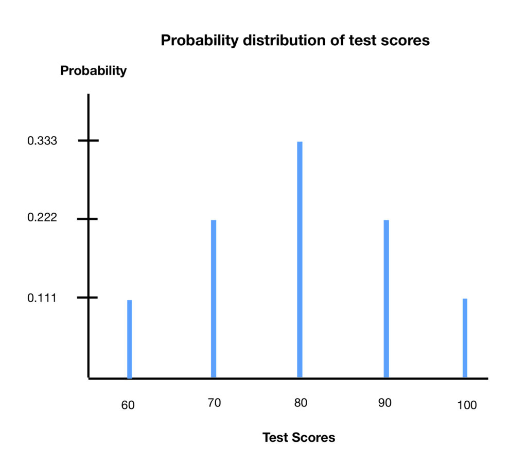
There are two things to note about the probability distribution:
First, the probabilities add up to 1 (since we’re expressing them as a decimal; if we were expressing them as percentages, then they would have to add up to 100%).

Second, if we multiply the value of the test score by it’s probability (expressed as a decimal) then we’ll wind up with the average (or mean) of the scores.
The mathematical shorthand for this is:
 where
where
 represents the probability of
  represents the values of the test scores
 is an index corresponding to one of the values in the table above
 is the maximum value of = the total # of test scores
So 
Putting in some numbers:

In Bell’s paper, the entity that’s being considered is , the values of the hidden variables. corresponds to  in the above formulas. In the discussion found in Bell’s Inequality 1, look at the distribution of results from that article (second column from the right). A summary is as follows:
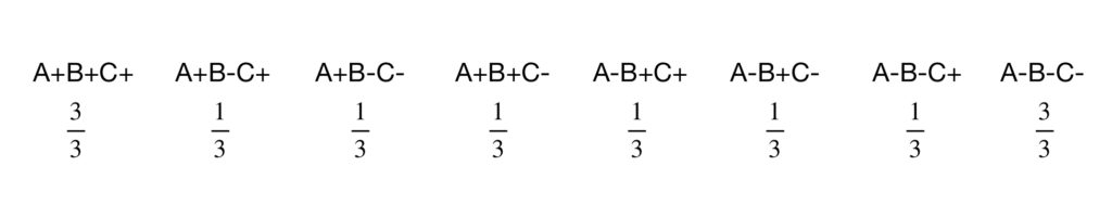
From the above table, we can see that there are 24 possibilities, 3 from each of the hidden variable programs (e.g., A+B-C+). A plot of probability of each of the hidden variable programs analogous to the probability plot for the test scores is shown below:
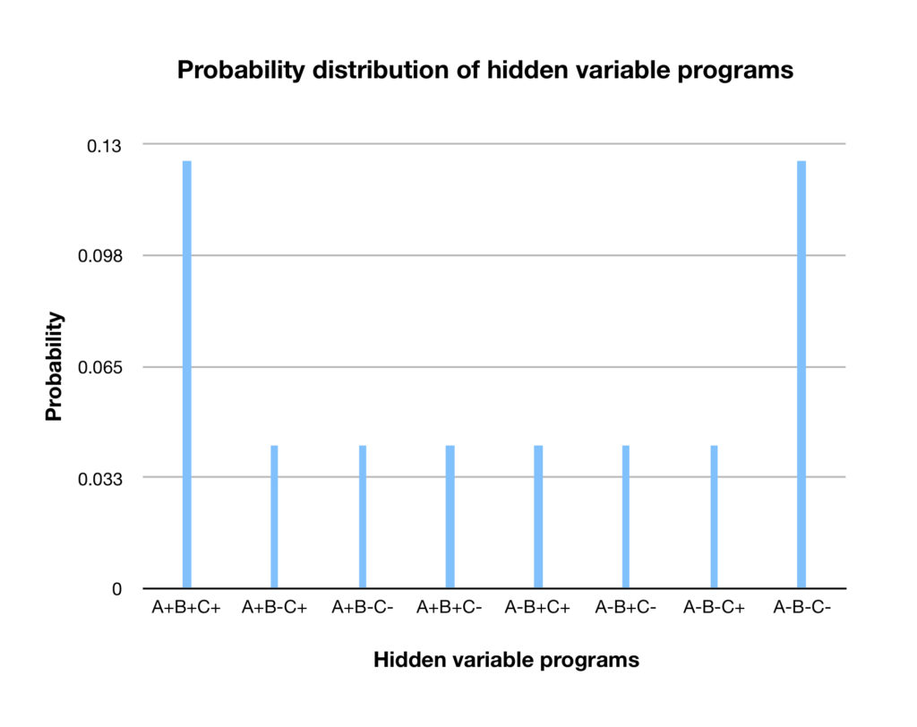
The probability plot shown above is for discrete variables. In the above chart, there are 8 discrete categories for which probabilities are plotted. In Bell’s paper, the variable for which the probabilities are plotted are continuous. In the experimental setup in the paper, the variable under consideration, , would be the hidden “program” that “tells” an entangled electron what measurement to assume at each angle at which a Stern-Gerlach device is pointed to measure it. It would be a number between 0˚ and 360˚-any number, not just integers-an infinite number of numbers. A plot of such a variable might look something like this:
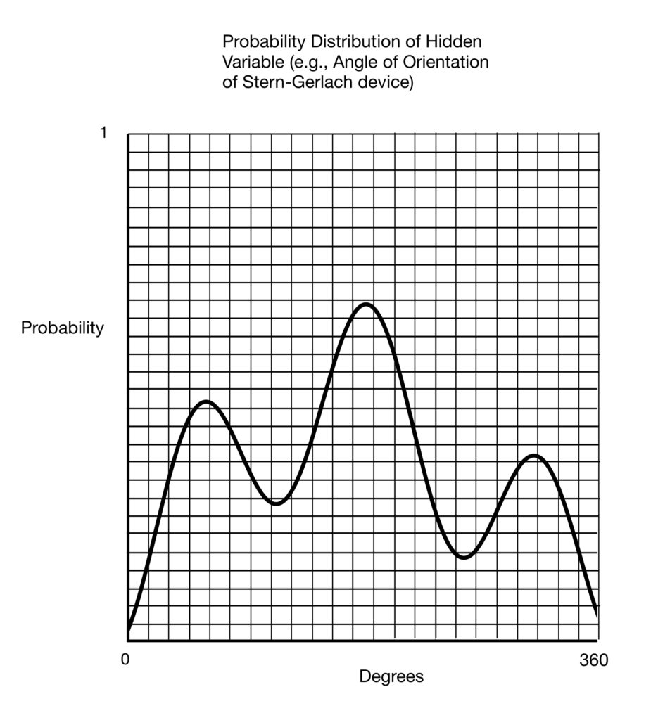
Figure 6
Since it’s a probability distribution, the total probability of occurrence of the hidden programs associated with “each degree” in the graph above, like the total probability in all of the other previously considered diagrams, add up to 1. But as we noted, the number of degrees and their associated probabilities that need to be considered with a continuous variable are infinite. So how do we calculate that total probability? The answer is “by use of an integral.”
Mathematical Interlude: The Integral
So what is an integral? An integral is a mathematical tool to find the area under a curve. To see how it works, consider the following diagram:
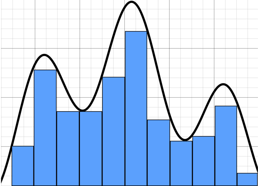
We can at least get an estimate of the area under the curve in the graph shown above by drawing rectangles. Note that, in the graph, there is a considerable amount of “white” between the blue rectangles and the curve. This indicates that the accuracy of our estimate is limited.
We can make our estimate better by making the rectangles we use to measure narrower, like so:
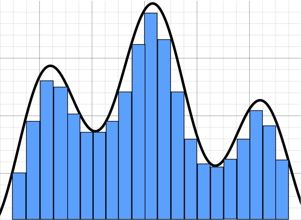
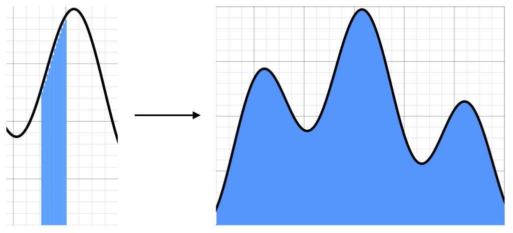
The above estimate looks better, with less white space. This suggests that if we continue to make our rectangles narrower and narrower, eventually making them infinitesimally small, we should eventually get the true area under the curve:
The above graphs can be described mathematically as follows:
 where
where 
In the above equation,
 is the value of the curve, specified on the y-axis.
  is an infinitesimal displacement along the x-axis.
  means multiply and together.
  is the integral sign. It means, find the area under the curve specified by and the axis that lies between
  and
and  .
. - The right side of the equation tells us how to find the integral on the left side of the equation.
 means that the right side of the equation is an approximation of the left side.
 - The manner in which this approximation is carried out is by adding up the area of a bunch of very narrow rectangles together-that is, take their sum. The mathematical symbols that tells us to take a sum is
 .
. - The thing that we’re to take the sum of is to the right of the symbol. In this case, the equation says to take the sum of the product of times
 at multiple sites along the axis.
 - The product
 gives the area under the very narrow rectangles.
 - tells us where along the axis to take those products.
- is the width of the rectangles whose areas we’re going to add up to approximate the integral. This is given by dividing
 (the length along the x-axis for which we’re going to measure the area under ) by , the number of tiny rectangles whose areas we’re going to add together.
 - The number below and on top of the sign are references to the various tiny rectangles we’re going to add up.
 refers to the first rectangle we’re going to use to contribute to our sum, under the left-most aspect of the curve.
 - is an integer that refers to the right-most rectangle we’re going to use.
The expression  is called a Riemann sum (named after Bernhard Riemann, the eighteenth century mathematician who invented it). Application of the above mathematical methods to figure 7 may make the way that these methods work more clear.
Figure 7 can be expressed mathematically as follows:
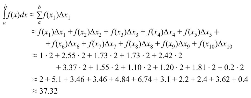
Here are a few comments of explanation regarding the above equations:
-
 is the value on the vertical (y) axis corresponding to the left-hand margin of the left-most first rectangle. It is the height of the rectangle.
  is the width of the base of that rectangle.
- The area of that rectangle is the height times the base, i.e.,
 .
. - Add up the areas of all of the rectangles and we have an estimate of the area under the curve.
We could go through the same exercise with figure 8 but it would be tedious and essentially the same as that given for figure 7. Therefore, let’s move on to figure 9 and give the mathematical expression for the exact value of the area under a curve:
 where
where
In this expression,  means that, in order to get an exact value for the area under the curve, , we would need to take the sum of the area of an infinite number of very narrow rectangles. As the above diagrams show, as the number of rectangles becomes very large-and their widths become very narrow-they “point to” the exact value.
We can apply the above mathematical technique to a probability distribution. By definition, a probability distribution is a cataloguing of the chances that a single event will unfold in a specific way. The event is destined to occur with 100% certainty. The percentages associated with each of the ways that the event can unfold, therefore, have to add up to 100%. Percentages can be converted to decimals by dividing the percentage by 100. The total percentage of the event happening can also be converted to a decimal: 100/100 = 1. The area of each of the little rectangles that we add up to to get the area under the probability distribution curve correspond to the probabilities we add up to get the total probability. The total probability, expressed as a decimal, is 1. Therefore, the area under the probability distribution curve is 1. I mention this fact now because it will come in handy at a later time in this article.
Proof (cont’)
Of course, the reason we went through the above primer on integrals is because they are an integral (pun intended) part of the remainder of the proof.
Let’s go back to the integral with which Bell begins:
Recall that and are measurements made widely separated in space. depends on the vector , the angle at which the measurement at is made, and , the hidden variable. depends on the vector , the angle at which the measurement at is made, and , the hidden variable. These measurements are both either plus or minus 1. And whatever the measurement at is, if the angle of measurement at both sites is the same, then the measurement at will be the opposite of that at . (As we shall see, fortunately, this is not necessarily the case if the angle of measurement at and are different.)
The above integral is analogous to a combination of 1) the calculation of the mean of a discrete probability distribution and 2) calculation of the area under a continuous probability distribution, described previously:
- is analogous to the value of on those probability distributions (i.e., the height of the infinitesimal rectangles that need to be added up)
 is the width of the base of those tiny rectangles
 is the area of the infinitesimal rectangles; if we add them all up we’ll get 1
- and are measurements;
 ; we’re working under the assumption that there is some program specified by the hidden variables, , that determines what and will be for each angle of measurement,
  and
and 
- For each value of , we multiply the product of and by the area of each of the little rectangles (which represents the probability of occurrence for each value of
 ). Like in the mean calculation of the discrete probability distribution, this gives us a weighted average, the average (or mean) of all of the
  and
and  .
. - That mean is the value on that left side of the equation,

Because the particles being measured at and are entangled, if measured at the same angle (i.e.,  ), the measurements should be the inverse of each other. If that angle of measurement is , then
Substituting this result into our original integral, we get


Now consider measuring at another angle given by another vector,  . Similar to the equation
is the equation

For the same reasons that  was found to equal
  so
so  . And thus,

Now subtract  from both sides of
![\begin{array}{rcl}P(\vec{a},\vec{b})-P(\vec{a},\vec{c})&=&-\int{d\lambda\rho(\lambda)A(\vec{a},\lambda)A(\vec{b},\lambda)}\,-\,\left[-\int{d\lambda\rho(\lambda)A(\vec{a},\lambda)A(\vec{c},\lambda)}\right]\\&=&-\int{d\lambda\rho(\lambda)A(\vec{a},\lambda)A(\vec{b},\lambda)}\,+\,\int{d\lambda\rho(\lambda)A(\vec{a},\lambda)A(\vec{c},\lambda)}\right]\\&=&\int{d\lambda\rho(\lambda)\left[-A(\vec{a},\lambda)A(\vec{b},\lambda)}+A(\vec{a},\lambda)A(\vec{c},\lambda)}\right]\\&=&\int{d\lambda\rho(\lambda)\left[A(\vec{a},\lambda)A(\vec{c},\lambda)}-A(\vec{a},\lambda)A(\vec{b},\lambda)}\right]\end{array}](https://www.samartigliere.com/wp-content/ql-cache/quicklatex.com-9850f0eabaf71625f283b3a178757d98_l3.png "Rendered by QuickLaTeX.com")
Note that  . This is because, if
  , then
  . Likewise, if
  , then
  .
.
Therefore,
![\begin{array}{rcl}A(\vec{a},\lambda)A(\vec{c},\lambda)&=&A(\vec{a},\lambda)\left[1\right]A(\vec{c},\lambda)\\&=&A(\vec{a},\lambda)\left[A(\vec{b},\lambda)(A(\vec{b},\lambda)\right]A(\vec{c},\lambda)\end{array}](https://www.samartigliere.com/wp-content/ql-cache/quicklatex.com-c97ec96499584ab6937407d0ceaf6eb3_l3.png "Rendered by QuickLaTeX.com")
Now substitute the lower row of the right-hand side of the above equation into our previous equation:
![\begin{array}{rcl}P(\vec{a},\vec{b})-P(\vec{a},\vec{c})&=&\int{d\lambda\rho(\lambda)\left[A(\vec{a},\lambda)A(\vec{c},\lambda)}-A(\vec{a},\lambda)A(\vec{b},\lambda)}\right]\\&=&\int{d\lambda\rho(\lambda)\left[A(\vec{a},\lambda)\left[A(\vec{b},\lambda)A(\vec{b},\lambda)\right]A(\vec{c},\lambda)-A(\vec{a},\lambda)A(\vec{b},\lambda)}\right]\\&=&\int{d\lambda\rho(\lambda)\left[\left(A(\vec{a},\lambda)A(\vec{b},\lambda)\right)\left(A(\vec{b},\lambda)A(\vec{c},\lambda)\right)-A(\vec{a},\lambda)A(\vec{b},\lambda)}\right]\end{array}](https://www.samartigliere.com/wp-content/ql-cache/quicklatex.com-24d822a1da5163b7d811065bf7e42d90_l3.png "Rendered by QuickLaTeX.com")
Next factor out  from the above equation. We get:
![P(\vec{a},\vec{b})-P(\vec{a},\vec{c})&=&\int{d\lambda\rho(\lambda)A(\vec{a},\lambda)A(\vec{b},\lambda)\left[A(\vec{b},\lambda)A(\vec{c},\lambda)}-1\right]](https://www.samartigliere.com/wp-content/ql-cache/quicklatex.com-b7b0bb824a1f90c6b7a6098a5380272b_l3.png "Rendered by QuickLaTeX.com")
Factor our -1. That leaves
![P(\vec{a},\vec{b})-P(\vec{a},\vec{c})&=&-\int{d\lambda\rho(\lambda)A(\vec{a},\lambda)A(\vec{b},\lambda)\left[1-A(\vec{b},\lambda)A(\vec{c},\lambda)}\right]](https://www.samartigliere.com/wp-content/ql-cache/quicklatex.com-dcfae65eb42fb9edb50387eae4b3254d_l3.png "Rendered by QuickLaTeX.com")
Recall that  and
and  . Below is a table that depicts what happens when we multiply
  and together:
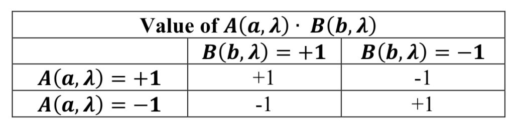
From the table, we can see that the maximum that  can be is +1 and the minimum it can be is -1. If or are less than +1 or greater than -1, then is between +1 and -1. Mathematically, this is expressed as:

There’s a function called the absolute value. It’s mathematical symbol is a vertical line to the left and right of the expression we want the absolute value of . When you take the absolute value of an expression, it makes the expression non-negative. So positive expressions remain positive, negative expressions turn positive, and expressions that evaluate to 0 remain 0. Another way to say this is that, when we take the absolute value of a number, we’re asking “on a number line, how far away from zero do we have to travel to get to the number.” For example, if you want to take the absolute value of 3 or -3, you would start at 0 and travel 3 units along the number line either in the positive or negative direction. The amount or magnitude of units you travel, disregarding the direction, is the absolute value:
In the left-hand portion of the equation above,  , we could make the equation true by traveling a distance less than or equal to 1 unit. Therefore, the absolute value of is less than 1. In mathematical terms:

Similarly, we could make the right-hand side of equation,  , true by traveling less than or equal to 1 unit. Therefore, the absolute value of is also less than or equal to 1:

So, starting from the equation , we’ve established that  . By similar reasoning,
  . Therefore,
  .
.
Next, take the absolute value of
That gives us
![\mid P(\vec{a},\vec{b})-P(\vec{a},\vec{c}) \mid\,\,&=&\,\,\mid-\int{d\lambda\rho(\lambda)A(\vec{a},\lambda)A(\vec{b},\lambda)\left[1-A(\vec{b},\lambda)A(\vec{c},\lambda)}\right] \mid](https://www.samartigliere.com/wp-content/ql-cache/quicklatex.com-7f229bb5344ce74a08180e887bc17c4d_l3.png "Rendered by QuickLaTeX.com")
The absolute value sign makes both sides of the equation positive.  is positive. If the magnitude of
  is less than one then that means that the absolute value of
  is some fraction of . Which means that must be greater than the absolute value of . On the other hand, if the magnitude of equals 1, then that means that the absolute value of is equal to . It follows, then, that
![\begin{array}{rcl}\mid P(\vec{a},\vec{b})-P(\vec{a},\vec{c})\mid \,\,&\leq&\,\,\int{d\lambda\rho(\lambda)\left[1-A(\vec{b},\lambda)A(\vec{c},\lambda)}\right]}\\&\leq& \int{d\lambda\rho(\lambda)(1)-\int\{d\lambda\rho(\lambda)A(\vec{b},\lambda)A(\vec{c},\lambda)}\\&\leq&1-\int\{d\lambda\rho(\lambda)A(\vec{b},\lambda)A(\vec{c},\lambda)}\end{array}](https://www.samartigliere.com/wp-content/ql-cache/quicklatex.com-5bc14300701684fc3136d4bee5010ca1_l3.png "Rendered by QuickLaTeX.com")
Now  . And for the same reasons that ,
  .
.
So

That’s the famous Bell inequality. It describes the expectation values anticipated from measurement of the spin of entangled electron pairs, under conditions where hidden variables predetermine the outcome of these measurements.
Significance of Bell’s Inequality
In the last part of his paper, Bell proves that the expectation values predicted by quantum mechanics differ from those predicted by his inequality (which, of course, is based on the kind of classical hidden variables theory that Einstein advocated). He does this by developing expressions for the difference in expectation values given by the Bell’s inequality and those given by quantum mechanics, then proves that that difference can never be zero. The proof is long and difficult. Its explanation would take longer than the one already provided above and that explanation is already too long. Therefore, we’ll consider a shorter, informal demonstration given by Griffin in his classic textbook on quantum physics3.
Imagine making measurements at 3 angles,  ,
,  .
.  . As Bell points out in the beginning of his paper, the expectation value for two such events occurring simultaneously is given by dot product between the angle at which the 2 measurements are made. And the dot product equals the cosine of the angle between the 2 measurements. This follows from the fact that the average value of a probability function (i.e., the mean, the expectation value) is equal to the sum (for discrete variables) or integral (for continuous values) of each measurement times the probability of the occurrence of that measurement. Remember? We had a discussion about this in the sections of this paper entitled Probability Distribution:
 where
where
 is the expectation value of
- For our purposes, is the product of the measurements that result when one entangled electron is measured at A at angle and its entangled partner is measured at B at angle ; or at A and at B; or at A and at B; or in each case, vice versa
 is the probability that occurs
From here, through a series of steps, we end up with the following relationships:
 ;
;  ;
;  ; where, for example
 represents the expectation value (i.e., average or mean) of the product of the measurements when one entangled electron is measured at A at angle and its entangled partner is measured at B at angle
  represents the dot product of and
It so happens that  where
where
 and
and  are the magnitude of and
  is the angle between and
 - The magnitude of a vector equals its absolute value; thus,

That means that 
It follows, then, that

But the entangled electrons we’re measuring are anti-correlated. Therefore, we need to add a minus sign to the right side of the equation:

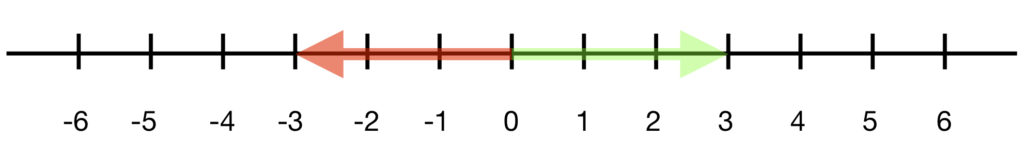
The proof of this is somewhat involved, requiring considerable background on quantum mechanics and the math associated with it. This is more than I wish to take on in this article. However, this information will be discussed in a subsequent article and a reference to that information will be subsequently be left here. In the meantime, the following diagram may provide an intuitive feel for this:
In the above diagram, vectors a, b and c have a magnitude of 1. represents measurement in the  direction. represents measurement in the
  direction. represents measurement in the
  direction. The vertical dotted line represents the projection of on (i.e., the component of in the direction). The horizontal dotted line represents the projection of on (i.e., the component of in the direction). And the projection of one vector on another is the dot products of those two vectors, which is the cosine of the angle between the vectors.
So, from the diagram
- The cosine of the angle between and equals zero. That’s because there is no component of in the direction of .
- The cosine of the angle between and equals
 . That’s because the component of in the direction of
  .
. - The cosine of the angle between and equals . =
 . That’s because the component of in the direction of .
Of course, as stated above, the spin of the entangled particles in Bell’s paper are anti-correlated. Therefore,


In Bell’s paper
- the expectation value of the product of measurements made of entangled photons at A in the direction and at B in the direction (
 ) is given by the expression
- the expectation value of the product of measurements made of entangled photons at A in the direction and at B in the direction (
 ) is given by the expression
From this, we get


According to Bell’s inequality

Putting in the above numbers:

 This is NOT true!
That means that the predictions of the classical local hidden variables theory on which Bell’s inequality is based do not agree with the predictions of quantum mechanics.
That was good news when it was discovered for it provided a way to test whether classical physics or quantum physics is correct. The above experiment could be done, and if results agreed with Bell’s inequality, then it would prove that there are local hidden variables at work. On the other hand, if results agreed with the predictions of quantum mechanics, it would indicate that quantum mechanics is correct.
So which is it? Which theory do results of the above experiment support? Well, now you’re probably going to throw eggs and rotten tomatoes at your screen because, at least to my knowledge, the above experiment has not been done. However, variants of the above experiment have been done that test different forms of Bell’s inequality. The results of these experiments are discussed in the next installment of this series, Bell’s Inequality III.
References
1. https://link.springer.com/article/10.1007%2FBF02728310
2. >https://en.wikipedia.org/wiki/Stern–Gerlach_experiment
3. Griffin, David J.“Introduction to Quantum Mechanics.” Introduction to Quantum Mechanics, Prentice Hall, 1995, p. 379.