Primer on Quantum Mechanics – Sam Artigliere's Blog

Introduction
Wave function
Basic principles of quantum mechanics
Spin
Experimental evidence
Mathematical description of spin
Other operators and wave functions

Introduction

It is useful to divide physics, specifically mechanics (the study of motion and forces), into two main categories: classical and quantum mechanics.

When we think of classical mechanics, for most people, Newtonian mechanics comes to mind since that is what is usually taught in high school and as a first course in undergraduate physics. But there are other formulations – like the Lagrangian, Hamiltonian and Hamilton-Jacobi formulations. These “alternative” formulations actually are more easily relatable to quantum mechanics than the Newtonian formulation, and as we shall see later in this article, are actually more pertinent to this discussion. However, all of these formulations of classical mechanics have one thing in common: if we know the position and velocity (or momentum since momentum equals mass x velocity) of all of the particles in an ensemble of particles at a given time, we will know their position and velocities at all times in the future. A corollary to this is that, if we have complete knowledge of the state of a system at one time, we can theoretically predict the results of any future event, including results of experiments, with certainty.

By contrast, in quantum mechanics, per the Heisenberg uncertainty principle, the position and velocity of a particle cannot be both known definitively at the same time. If the position is known definitively then the we can’t know the velocity(momentum) and visa vera. Similarly, the results of individual experiments cannot be predicted definitively. Instead, only the probability of an outcome can be predicted before an experiment is run. However, if the experiment is performed a large number of times, the percentages of occurrence of various outcomes approaches those predicted by classical mechanics.

Wave function

Newton developed his system of mechanics by looking at experimental results and developing equations to fit the data. Likewise, a mathematical framework was developed to fit the experimental findings in quantum mechanics.

One of the primary mathematical tools used to describe quantum mechanical phenomena is the wave function. The wave function is basically a vector or vector-like mathematical object such as a function that describes the state of a quantum mechanical system given a specific basis. Vectors, in the traditional sense of a finite collection of numbers, are used when we’re working with discrete variables like values of electron spin. Functions are used when working with continuous variables like particle position. Let’s consider traditional vectors because they convey the basic concepts better. Each component that makes up the wave function vector is called a probability amplitude and is a complex number. Each probability amplitude relates to (but is not the same thing as) the probability of a specific measurement occurring. To get the actual probability, we need to multiply the probability amplitude by its complex conjugate. The reason that complex numbers are used is not simple to explain. However, the basic idea is that quantum mechanics deals with waves that not only have magnitude but also have phase. It is this phase factor that leads to constructive and destructive interference of these waves which leads to the very different behavior of quantum objects as compared with classical objects. The use of complex numbers introduces this phase factor. (Think of the hand of a clock pointing in various directions. The length of the hand represents the magnitude of a vector. The directions in which the hand points represents the phase. However, no matter in which direction the hand points, its length, i.e., magnitude, remains the same.)

Basic principles of quantum mechanics

Many of the additional key points of the mathematical framework of quantum mechanics can be expressed in a group of four principles or postulates. Linear algebra plays a significant role in these postulates. We will state them first then attempt to explain them after. Most of this discussion comes from an excellent book written by renowned Stanford physicist Leonard Susskind and his coauthor Art Friedman, geared toward the interested amateur. The book can be obtained at the following link:

https://www.amazon.com/Quantum-Mechanics-Theoretical-Leonard-Susskind/dp/0465062903/

Susskind also has a fantastic series of lectures on physics called The Theoretical Minimum. It the can be found here.

Getting back to our subject, the 4 postulates of quantum mechanics are:

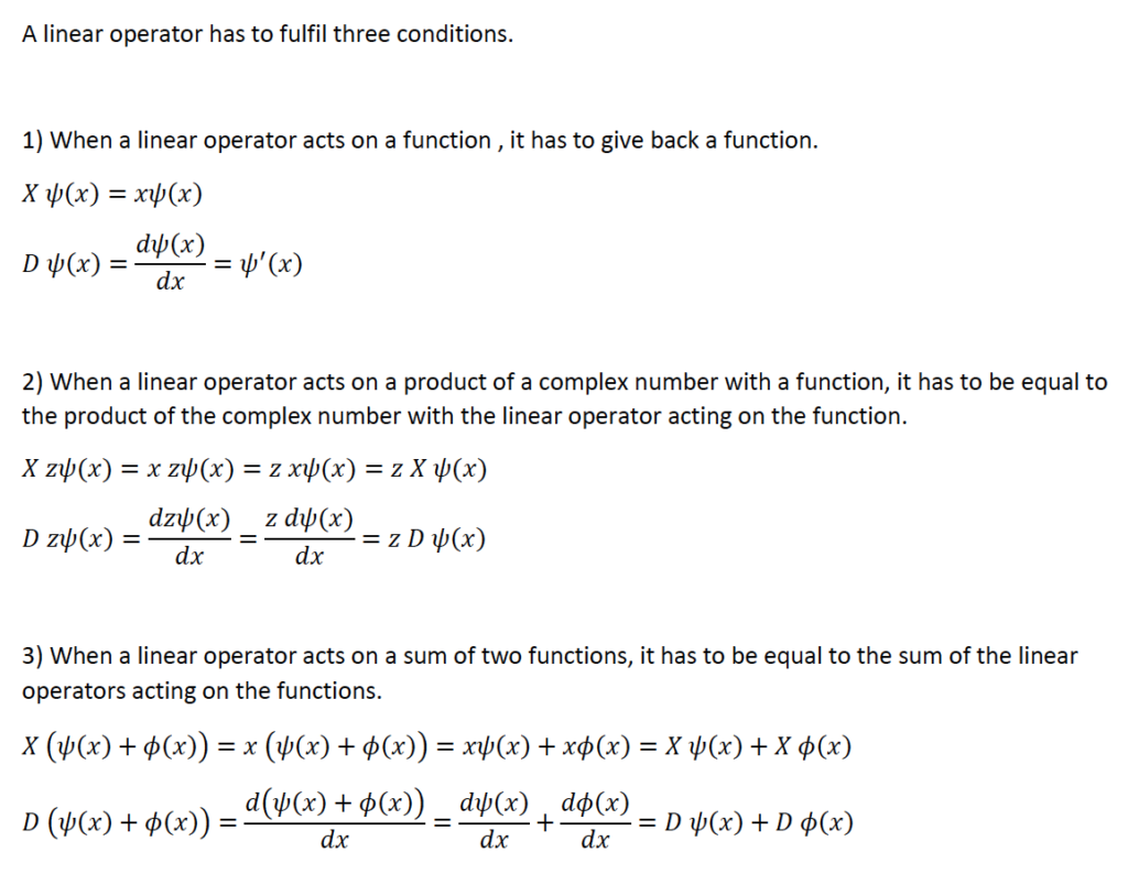
The observable or measurable quantities of quantum mechanics (like spin, position, momentum and energy of particles) are represented by linear operators. These are essentially Hermitian matrices, mathematical objects that fall within the subject of linear algebra.
The possible results of a measurement are the eigenvalues, $\lambda_i$ , of the operator that represents an observable. The state for which the result of a measurement is unambiguously $\lambda_i$ is the corresponding eigenvector, $\ket {\lambda_i}$ .
Unambiguously distinguishable states are represented by orthogonal vectors.
If $\ket {A}$ is at the state vector of a system, and the observable $L$ is measured, the probability to observe measurement value $\lambda_i$ is

$P(\lambda_i) = \braket{A}{\lambda_i} \braket{\lambda_i}{A}$

Spin

We will use the spin of an electron as an example to illustrate how the above-described mathematical machinery works.

Electron spin is a purely quantum phenomenon that has no direct correlate with classical mechanics. The closest we can come to a classical model for spin is to think of a charged particle spinning on its central axis, creating a magnetic field and acting as a tiny bar magnet. If we were to curl our second through fifth fingers in the direction of a particle’s rotation, the direction in which our thumb points would give us the direction of the north pole of the little bar magnet. (This is called the right-hand rule.) Mathematically, the closest classical approximation we have to spin is to consider it like rotational angular momentum intrinsic to a charged particle. Spin is the property that determines behavior of a particle in a magnetic field. Just as there are two directions in which a particle can spin, there are two (and only two) values that the spin of an electron can take: spin up and spin down. We’ll explain this in a minute.

If we place the electron in a constant external magnetic field, the electron, in terms of classical mechanics, will orient itself such that its north pole aligns with the direction of the magnetic field and its south pole against it. In quantum mechanical terms, if the electron spin is aligned with the magnetic field, it is spin up. If it is aligned opposite the magnetic field, it is spin down.

Now suppose we have an apparatus that can measure whether the electron is spin up or spin down. Details about how such an apparatus might accomplish this can be found here, but we won’t worry about that now. For our current purposes, we’ll just assume that it works. We also have a second apparatus that creates a magnetic field, causes an electron spin to align with its magnetic field (called preparing an electron), then transfers it to the measuring apparatus. (Again, for our purposes, it’s not important how this is carried out.) In what follows, we’ll assume that our electrons and our machines are located in a standard Cartesian coordinate with 3 orthogonal axes (i.e., oriented at right angles to one another) which we’ll call $x$ , $y$ and $z$ .

Experimental evidence

We’re going to start by considering the results of some experiments performed on the above-described equipment then we’ll try to come up with some equations that describe the data.

The axis conventions we’ll use for these experiments are as follows:

The plain of this page is the $x-z$ plane.
The $y$ axis goes in and out of this paper.
The $+z$ direction is up; the $-z$ direction is down.
The $+x$ direction is to the right; the $-x$ direction is to the left.
The $+y$ direction is away from us; the $-y$ direction is toward us.

First, prepare an electron with its spin up in the $+z$ -direction. Send it over to our measuring apparatus and measure it in the $+z$ -direction. If the spin is aligned with the magnetic field (i.e., it is spin up) then the apparatus will measure +1. If the spin is aligned against the magnetic field (i.e., it is spin down), then the apparatus will measure -1. Since the electron we prepared is spin up, the apparatus will measure +1, with 100% certainty. Another way of stating this is: if we prepare an infinite number of electrons in the spin up configuration, then every time we measure, our apparatus will measure +1. If we prepare another electron spin down, our apparatus will measure -1 with 100% certainty.

But what happens if we prepare the spin with its north pole pointing in the $+x$ -direction of space and measure with our apparatus pointing in the $+z$ -direction of space? Then with 50% probability, our apparatus will measure +1 and with 50% probability, it will measure -1. Said another way, if we prepare an infinite number of electrons with spin in the $+x$ -direction and measure them with our apparatus oriented in the $+z$ direction, then 50% of the time our apparatus will measure +1 and 50% of the time, our apparatus will measure spin down. If we repeat the experiment a large but less than an infinite number of times, the results will approach a 50-50 split between +1 and -1 measurements.

If we prepare our spin at an angle of $30^{\circ}$ from the $+z$ -axis toward the $+x$ -axis and measure along the $+z$ axis, approximately 93.3% of the time, we will measure +1 and approximately 16.7% of the time we will measure -1.

Mathematical description of spin

Now for the mathematics that represent these results.

First, we said that the state of a system is specified by a state vector. If we specify a basis for the vector space we’re working with, then that state vector would represent a wave function. The basis for the vector space is determined by the measurement that we want to make. For example, suppose our measurement apparatus is oriented along the $z$ -axis and will measure spin up (i.e., +1) if an electron’s north pole is oriented in the $+z$ direction. Then the basis we will be measuring in we might call the $z$ basis. If a spin’s north pole is oriented in $+z$ direction, then it will be measured as $+1$ 100% of the time in this basis and its state will be referred to as $\ket{u}$ . If, on the other hand, a spin’s north pole is oriented in $-z$ direction, then it will be measured as $-1$ 100% of the time in this basis and its state will be referred to as $\ket{d}$ .

The state vector (call it $\ket{A}$ ) can be represented as

$\ket{A}=\alpha_u\ket{u}+\alpha_d\ket{d}$

where

$\alpha_u$ is the probability amplitude for the spin being in state $\ket{u}$
$\alpha_d$ is the probability amplitude for the spin being in state $\ket{d}$

Now

$\alpha_u^*$ is the complex conjugate of $\alpha_u$
$\alpha_d^*$ is the complex conjugate of $\alpha_d$

In turn

$\alpha_u=\braket{u}{A}$ . This is the dot product of $\bra{u}$ and $\ket{A}$ which represents the component of probability amplitude of $\ket{A}$ in the direction of $\ket{u}$ .
$\alpha_d=\braket{d}{A}$ . This is the dot product of $\bra{d}$ and $\ket{A}$ which represents the component of probability amplitude of $\ket{A}$ in the direction of $\ket{d}$ .

Thus, if

$P_u$ represents the probability of spin being spin up
$P_d$ represents the probability of spin being spin down

then

$P_u=\alpha_u^*\alpha_u$
$P_d=\alpha_d^*\alpha_d$

For some intuition as to why this is so, click :

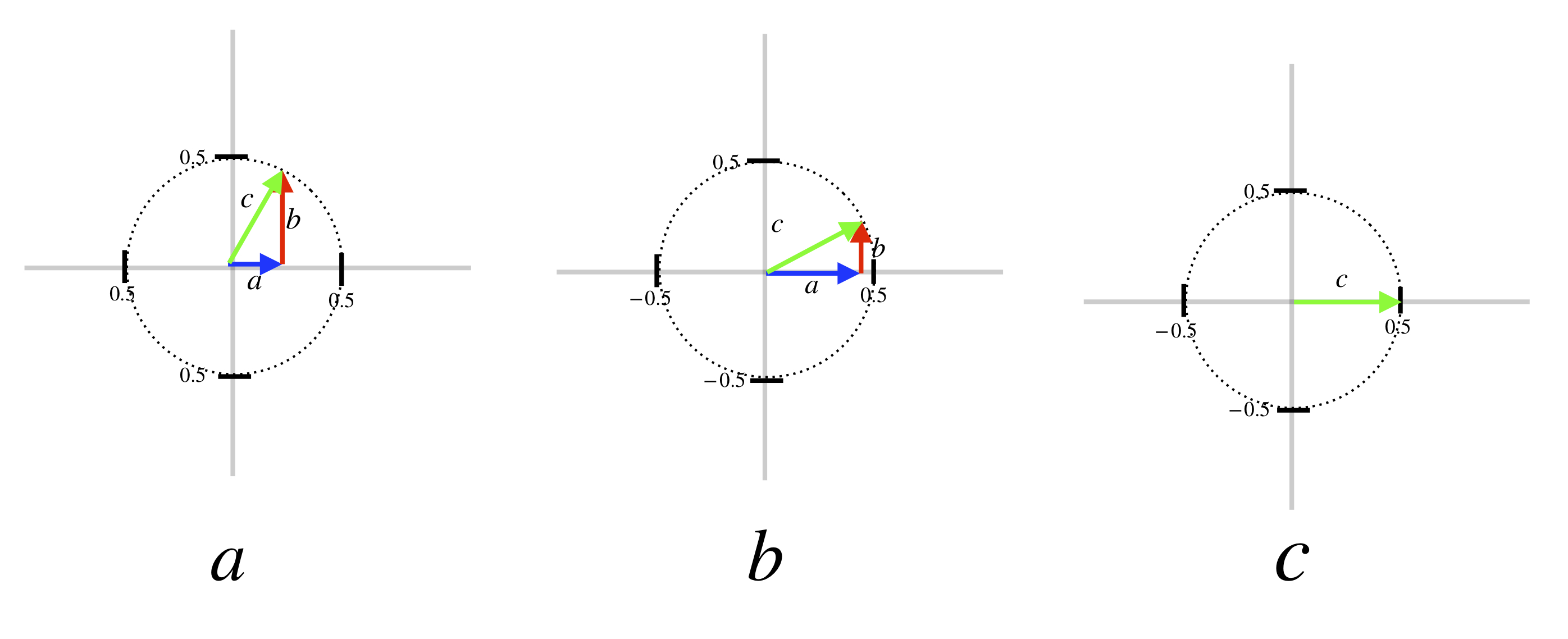
As we said, probability in quantum mechanics is represented by vectors. The entities that are represented along the axes of the coordinate system on which these vectors are constructed are probability amplitudes. They form the basis for the vector space of which these probability vectors are a part. In the case of the spins we’ve been talking about, spin up, for example, can be represented on one axis and spin down on the other, as shown in the diagram.

Since $\alpha_u=\braket{u}{A}$ and $\alpha_d=\braket{d}{A}$ ,

this is just a restatement of the fourth basic principle of quantum mechanics:

$P(\lambda_i) = \braket{A}{\lambda_i} \braket{\lambda_i}{A}$

In this case, the eigenvector, $\lambda_i$ , is either $\ket{u}$ and $\ket{d}$ . So

$P(u) = \braket{A}{u} \braket{u}{A}$
$P(d) = \braket{A}{d} \braket{d}{A}$

It should also be noted that the sum of all of the probabilities have to add to 1. That is,

$P_{total} = P_u + P_d = \alpha_u^*\alpha_u + \alpha_d^*\alpha_d=1$

If the reason for this is not clear, an explanation can be found .

Spin prepared in Z and measured in z

Now let’s move on to explaining some experimental results.

If we prepare an electron in the spin up position, then with 100% certainty, the spin will be measure as +1 by our apparatus. Therefore,

$\alpha_u=1+0i=1$
$\alpha_d=0+0i=0$
$\alpha_u^*=1+0i=1$
$\alpha_d^*=0-0i=0$

and

$P_u=\alpha_u^*\alpha_u=1\cdot1=1$
$P_d=\alpha_d^*\alpha_d=0\cdot0=0$

We could also say that $\ket{A}=1\ket{u}+0\ket{d}=\ket{u}$ .

Another way to represent the state vectors described above is via a column vector with the top entry representing the probability amplitude associated with being spin up and the bottom column representing the probability amplitude associated with being spin down. Thus,

If electron spin is up in the $+z$ direction, then $\ket{A}=\mqty[ 1\\0]$
If electron spin is down in the $+z$ direction, then $\ket{A}=\mqty [0\\1]$

Using the same conventions, if a spin is prepared with its north pole pointing in the $-z$ direction and and our measuring device is oriented in the $+z$ direction, then

$\ket{A}=\alpha_u\ket{u}+\alpha_d\ket{d}=0\ket{u}+1\ket{d}=\ket{d}=\mqty [0\\1]$
$\alpha_u=0+0i=0$
$\alpha_d=1+0i=1$
$\alpha_u^*=0+0i=0$
$\alpha_d^*=1-0i=1$
$P_u=\alpha_u^*\alpha_u=0\cdot0=0$
$P_d=\alpha_d^*\alpha_d=1\cdot1=1$

Note that quantum principle 3 states that $\ket{u}$ and $\ket{d}$ form an orthonormal basis. The “ortho” part of this expression means that these 2 vectors are orthogonal which means that their dot product should equal 0. If we check

$\braket{d}{u} = \mqty[0 & 1]\mqty[1\\0]=1 \cdot 0 +0 \cdot 1 = 0+0=0$

which confirms our supposition.

It may seem peculiar that $\braket{d}{u}$ , the dot product between $\bra{d}$ and $\ket{u}$ is zero since

the dot product is supposed to be zero only when two vectors are orthogonal
orthogonal vectors are usually thought of as being oriented at $90^\circ$ to each other
but the spins represented by $\bra{d}$ and $\ket{u}$ appear to be oriented at $180^\circ$ to each other

Well, it is true that the spin up and spin down are oriented at $180^\circ$ to each other in space. However, the thing that’s being plotted on the axis and abscissa to get the probability vector is probability amplitude, not direction in space, and the axes for these probability amplitudes are orthogonal (i.e., can be thought of as being perpendicular to each other), as depicted in the diagram below:

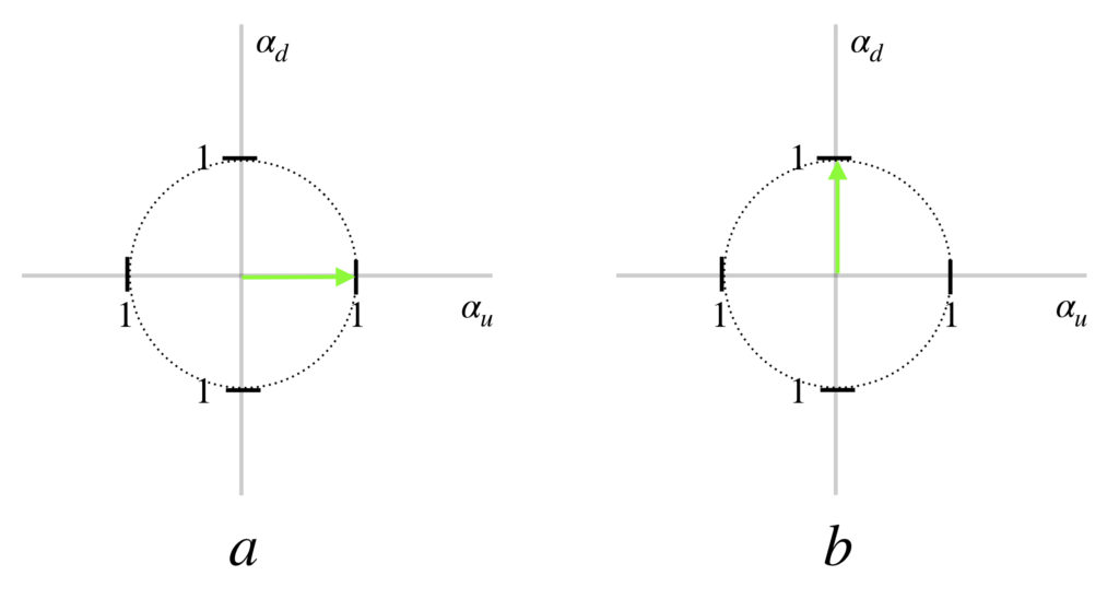
In the diagrams above, the entity described on the axes are probability amplitude. The probability amplitude associated with a spin being in the up spatial direction is purposely displayed on the horizontal axis to emphasize that what is being plotted here is not spatial direction. In a the probability amplitude is 100% spin up which means the probability of measuring the spin in the spin up direction is $1^2=1$ (i.e., 100%). In b, the probability amplitude is 100% spin down which means the probability of measuring the spin in the spin down direction is $1^2=1$ (i.e., 100%).

Spin prepared in X and measured in x

We can have a discussion which is similar to the one we just had if an electron spin is prepared in the $+x$ direction, leading to state $\ket{r}$ , and our measuring device is oriented in the $+x$ direction. If this is so, then

$\ket{r}$ means that electron spin is oriented in the $+x$ with 100% certainty
$\ket{l}$ means that electron spin is oriented in the $-x$ with 100% certainty

and

$\ket{A}=\alpha_r\ket{r}+\alpha_l\ket{l}$

where

$\alpha_r$ is the probability amplitude for the spin being in state $\ket{r}$
$\alpha_l$ is the probability amplitude for the spin being in state $\ket{l}$

Analogous to the previous case

$\alpha_r^*$ is the complex conjugate of $\alpha_r$
$\alpha_l^*$ is the complex conjugate of $\alpha_l$

$P_r$ represents the probability of spin being spin up
$P_l$ represents the probability of spin being spin down

then

$P_r=\alpha_r^*\alpha_r$
$P_l=\alpha_l^*\alpha_l$

If we prepare an electron in the spin up position, then with 100% certainty, the spin will be measure as +1 by our apparatus. Therefore,

$\alpha_r=1+0i=1$
$\alpha_l=0+0i=0$
$\alpha_r^*=1+0i=1$
$\alpha_l^*=0-0i=0$

and

$P_r=\alpha_r^*\alpha_r=1\cdot1=1$
$P_l=\alpha_l^*\alpha_l=0\cdot0=0$

We could also say that $\ket{A}=1\ket{r}+0\ket{l}=\ket{r}$

If we prepare a spin in the $-x$ direction and measure in the $+x$ direction, then by arguments similar to the case where a spin is prepared in the $-z$ direction and measured in the $+z$ direction:

$\ket{A}=0\ket{r}+1\ket{l}$
$P_r=\alpha_r^*\alpha_r=0\cdot0=0$
$P_l=\alpha_l^*\alpha_l=1\cdot1=1$

spin prepared in x and measured in z

Next, let’s prepare a spin in the $+x$ direction and measure it in the $+z$ direction. Preparation in the $+x$ direction leads to state $\ket{r}$ which means that, with 100% certainty, the spin has its north pole pointing in the $+x$ direction. Since we’re measuring in the $z$ basis, the wave function of that describes the state of our spin has got to be expressed in the $z$ basis (i.e., as a linear combination of $\ket{u}$ and $\ket{d}$ ). To fit the data from experimental results, the state of our spin must be

$\ket{A}=\frac{1}{\sqrt{2}}\ket{u}+\frac{1}{\sqrt{2}}\ket{d}$

This means that

The probability amplitude associated with the spin being measured as $+1$ is $\alpha_u=\frac{1}{\sqrt{2}}$
The probability amplitude associated with the spin being measured as $-1$ is $\alpha_d=\frac{1}{\sqrt{2}}$

Since $P_u$ , the probability of the measurement being $+1$ is given by

$P_u=\alpha_u^*\alpha_u$

then

$P_u=\frac{1}{\sqrt{2}}\frac{1}{\sqrt{2}}=\frac{1}{2}$

For a spin prepared in the $-x$ direction leading to state $\ket{l}$ and measured in the $+z$ direction, again, 50% of the time we will measure +1 and 50% of the time, -1. An equation that fits this data is

$\ket{l} = \frac{1}{\sqrt{2}}\ket{u} - \frac{1}{\sqrt{2}}\ket{d}$

The reason for the minus sign is that, like $\ket{u}$ and $\ket{d}$ , $\ket{r}$ and $\ket{l}$ form an orthonormal basis which means that their dot product equals zero. The only way that this can happen is if $\ket{l} = \frac{1}{\sqrt{2}}\ket{u} - \frac{1}{\sqrt{2}}\ket{d}$ . Here is the calculation:

$\begin{array}{rcl} \braket{l}{r} &=& (\frac{1}{\sqrt{2}}\bra{u} + \frac{1}{\sqrt{2}}\bra{d}) (\frac{1}{\sqrt{2}}\ket{u} - \frac{1}{\sqrt{2}}\ket{d})\\ &=& \frac{1}{\sqrt{2}}\frac{1}{\sqrt{2}}\braket{u}{u} - \frac{1}{\sqrt{2}}\frac{1}{\sqrt{2}}\braket{u}{d} + \frac{1}{\sqrt{2}}\frac{1}{\sqrt{2}}\braket{d}{u} - \frac{1}{\sqrt{2}}\frac{1}{\sqrt{2}}\braket{d}{d} \end{array}$

Because $\ket{u}$ and $\ket{d}$ form an orthonormal basis

$\ket{u}$ and $\ket{d}$ are orthogonal $=>$ their dot product is zero: $\braket{u}{d} = \braket{d}{u} =0$
$\ket{u}$ and $\ket{d}$ are normalized $=>$ their dot product is 1: $\braket{u}{u} = \mqty[1&0]\mqty[1\\0] = 1 + 0 = 1\text{;}\quad\braket{d}{d} =\mqty[0&1]\mqty[0\\1] = 0 + 1 = 1$

Therefore,

$\begin{array}{rcl} \braket{l}{r} &=& \frac{1}{\sqrt{2}}\frac{1}{\sqrt{2}}\braket{u}{u} - \frac{1}{\sqrt{2}}\frac{1}{\sqrt{2}}\braket{u}{d} + \frac{1}{\sqrt{2}}\frac{1}{\sqrt{2}}\braket{d}{u} - \frac{1}{\sqrt{2}}\frac{1}{\sqrt{2}}\braket{d}{d}\\ &=& \frac12 \cdot 1 - \frac12 \cdot 0 + \frac12 \cdot 0 - \frac12 \cdot 1 \\ &=& \frac12 - 0 + 0 - \frac12 \\ &=& 0 \end{array}$

$\ket{l} = \frac{1}{\sqrt{2}}\ket{u} - \frac{1}{\sqrt{2}}\ket{d}$

From this, we know that the probability amplitude associated with a -1 measurement is

$\alpha_d = \alpha_d^* = -\frac12$

Thus,

$P_d=\alpha_d^*\alpha_d=(-\frac{1}{\sqrt{2}})(-\frac{1}{\sqrt{2}})=\frac{1}{2}$

spin prepared at 30 ° from z and measured in z

So what happens if we prepare a spin with spin up in a direction $30^\circ$ clockwise from the $z$ -axis in the $x-z$ plane and measure in the $+z$ direction? This is a little more involved and will first require a discussion of linear operators, eigenvalues and eigenvectors. To understand this discussion, one needs to have a basic understanding of linear algebra. The previous section on requisite mathematics offers a brief presentation of this topic. A more extensive discourse on linear algebra can be found here.

Linear operators

Let’s begin by talking about linear operators. They are Hermitian matrices. They represent the entity to be measured. The eigenvalues of this matrix are the measurements. The eigenvectors of the linear operator matrix form the basis for a vector space. The eigenvectors also represent the quantum states that go along with each given measurement.

3 linear operators are associated with the measurement of electron spin, one for each spatial direction. We’ll call these $\sigma_z$ , $\sigma_x$ , and $\sigma_y$ . Let’s derive the expression for $\sigma_z$

Deriving σ_z

We know that the 2 possible measurements we can make are +1 and -1. So we know that the eigenvalues of $\sigma_z$ are +1 and -1. We know that the +1 eigenvalue is associated with the state $\ket{u}$ and -1 with $\ket{d}$ . That means that $\ket{u}$ and $\ket{d}$ are the eigenvectors. We can represent these facts by 2 equations:

$\mqty [(\sigma_z)_{11} & {(\sigma_z)}_{12} \\ {(\sigma_z)}_{21} & {(\sigma_z)}_{22}] \mqty [1 \\ 0] = +1\mqty [1 \\ 0]$

and

$\mqty[{(\sigma_z)}_{11} & {(\sigma_z)}_{12} \\ {(\sigma_z)}_{21} & {(\sigma_z)}_{22}] \mqty [0 \\ 1] = -1\mqty [0 \\ 1]$

This gives us 4 equations with 4 unknowns:

$\begin{array}{rcl} (1)(\sigma_z)_{11} + (0){(\sigma_z)}_{12} &=& 1 \quad \Rightarrow (\sigma_z)_{11} = 1 \\ \, &\,& \, \\ (1){(\sigma_z)}_{21} + (0){(\sigma_z)}_{22} &=& 0 \quad \Rightarrow (\sigma_z)_{21} = 0 \\ \, &\,& \, \\ (0){(\sigma_z)}_{11} + (-1){(\sigma_z)}_{12} &=& 0 \quad \Rightarrow (\sigma_z)_{12} = 0 \\ \, &\,& \, \\ (0){(\sigma_z)}_{21} + (-1){(\sigma_z)}_{22} &=& 1 \quad \Rightarrow (\sigma_z)_{22} = -1 \end{array}$

Therefore,

$\sigma_z = \mqty [1 & \,\,\,\,\,0 \\ 0 & -1]$

We can derive $\sigma_x$ and $\sigma_y$ in a similar fashion. We’ll start with $\sigma_x$

Deriving σ_x

Recall that when we prepared a spin in the $+x$ direction and measured in the $+x$ direction we measured $+1$ and when we prepared a spin in the $-x$ direction and measured in the $+x$ direction we measured $-1$ . These facts can be expressed mathematically as

$\sigma_x \ket{r} = +1 \ket{r}$

and

$\sigma_x \ket{l} = -1 \ket{l}$

where

$\sigma_x$ is the matrix we’re trying to find
$\ket{r}$ is the state where the spin of the electron is definitely in the $+x$ direction
$\ket{l}$ is the state where the spin of the electron is definitely in the $-x$ direction

We know from our previous description of experiments that when we prepare an electron spin in the $+x$ and measure in the $+z$ direction, our apparatus measures +1 half the time and -1 half the time. So

$\ket{r} = \frac{1}{\sqrt 2}\ket{u} + \frac{1}{\sqrt 2}\ket{d}$

$\ket{l} = \frac{1}{\sqrt 2}\ket{u} - \frac{1}{\sqrt 2}\ket{d}$

The two equations above describe what are called linear superpositions. What it means, according to the standard (Copenhagen) interpretation of quantum mechanics, is that the spin of the electron is in an indeterminate state in which it is spin up and spin down simultaneously – a state in which it remains until it is measured. Then when it’s measured, it definitively assumes one of the two states, a phenomenon that is called the collapse of the wave function. This behavior of a particle one way while it isn’t being measured and another way when it is measured was one of the things that motivated Bohm to seek an alternative to the standard interpretation of quantum mechanics.

At any rate, returning to our equations, we substitute the appropriate column vectors for $\ket{u}$ and $\ket{d}$ . When we do, we get

$\ket{r} = \frac{1}{\sqrt 2}\mqty[1 \\ 0] + \frac{1}{\sqrt 2}\mqty[0 \\ 1]=\mqty[\frac{1}{\sqrt 2} \\ 0] + \mqty[0 \\ \frac{1}{\sqrt 2}]= \mqty[\frac{1}{\sqrt 2} \\ \frac{1}{\sqrt 2}]$

$\ket{l} = \frac{1}{\sqrt 2}\mqty[1 \\ 0] + \frac{1}{\sqrt 2}\mqty[\,\,\,\,\, 0 \\ -1]=\mqty[\frac{1}{\sqrt 2} \\ 0] + \mqty[\,\,\,\,\, 0 \\ -\frac{1}{\sqrt 2}]= \mqty[\,\,\,\,\, \frac{1}{\sqrt 2} \\ -\frac{1}{\sqrt 2}]$

We can use these facts to write 2 eigenvalue equations that look like this:

$\mqty [(\sigma_x)_{11} & {(\sigma_x)}_{12} \\ {(\sigma_x)}_{21} & {(\sigma_x)}_{22}] \mqty[\frac{1}{\sqrt 2} \\ \frac{1}{\sqrt 2}] = +1\mqty[\frac{1}{\sqrt 2} \\ \frac{1}{\sqrt 2}]$

and

$\mqty[{(\sigma_x)}_{11} & {(\sigma_x)}_{12} \\ {(\sigma_x)}_{21} & {(\sigma_x)}_{22}] \mqty[\,\,\,\,\, \frac{1}{\sqrt 2} \\ -\frac{1}{\sqrt 2}] = -1\mqty[\,\,\,\,\, \frac{1}{\sqrt 2} \\ -\frac{1}{\sqrt 2}]$

We can translate these eigenvalue equations into 4 equations in 4 unknowns:

$\begin{array}{rcl} \frac{1}{\sqrt 2}(\sigma_x)_{11} + \frac{1}{\sqrt 2}{(\sigma_x)}_{12} &=& \frac{1}{\sqrt 2} \quad \Rightarrow (\sigma_x)_{11} = \frac{1}{\sqrt 2} \\ \, &\,& \, \\ \frac{1}{\sqrt 2}{(\sigma_x)}_{21} + \frac{1}{\sqrt 2}{(\sigma_x)}_{22} &=& \frac{1}{\sqrt 2} \quad \Rightarrow (\sigma_x)_{21} = \frac{1}{\sqrt 2} \\ \, &\,& \, \\ \frac{1}{\sqrt 2}{(\sigma_x)}_{11} - \frac{1}{\sqrt 2}{(\sigma_x)}_{12} &=& -\frac{1}{\sqrt 2} \quad \Rightarrow (\sigma_x)_{12} = \frac{1}{\sqrt 2} \\ \, &\,& \, \\ \frac{1}{\sqrt 2}{(\sigma_x)}_{21} - \frac{1}{\sqrt 2}{(\sigma_x)}_{22} &=& \frac{1}{\sqrt 2} \quad \Rightarrow (\sigma_x)_{22} = \frac{1}{\sqrt 2} \end{array}$

Add the first and third equations. That gives us

$\begin{array}{cccccc} & \frac{1}{\sqrt 2}(\sigma_x)_{11} & + & \frac{1}{\sqrt 2}{(\sigma_x)}_{12} &=& \frac{1}{\sqrt 2}\\ + & \frac{1}{\sqrt 2}{(\sigma_x)}_{11} & - & \frac{1}{\sqrt 2}{(\sigma_x)}_{12} & = & -\frac{1}{\sqrt 2}\\ \hline &(\frac{1}{\sqrt 2} + \frac{1}{\sqrt 2}){(\sigma_x)}_{11} &+& (\frac{1}{\sqrt 2} - \frac{1}{\sqrt 2}){(\sigma_x)}_{12} &=& \frac{1}{\sqrt 2} - \frac{1}{\sqrt 2}\\ \, & \, & \, & \, & \, & \, \\ & (\frac{1}{\sqrt 2} + \frac{1}{\sqrt 2}){(\sigma_x)}_{11} &+& 0 &= &0 \\ & {(\sigma_x)}_{11} &\,& \, &= &0 \end{array}$

Substituting ${(\sigma_x)}_{11}=0$ back into the first equation gives:

$\begin{array}{ccccc} 0 &+& (\frac{1}{\sqrt 2}){(\sigma_x)}_{12} &=& \frac{1}{\sqrt 2}\\ \, &\,& {(\sigma_x)}_{12} &=& 1 \end{array}$

Next, add the second and fourth equations. That yields

$\begin{array}{cccccc} & \frac{1}{\sqrt 2}(\sigma_x)_{21} & + & \frac{1}{\sqrt 2}{(\sigma_x)}_{22} &=& \frac{1}{\sqrt 2}\\ + & \frac{1}{\sqrt 2}{(\sigma_x)}_{21} & - & \frac{1}{\sqrt 2}{(\sigma_x)}_{22} & = & \frac{1}{\sqrt 2}\\ \hline &(\frac{1}{\sqrt 2} + \frac{1}{\sqrt 2}){(\sigma_x)}_{11} &+& (\frac{1}{\sqrt 2} - \frac{1}{\sqrt 2}){(\sigma_x)}_{12} &=& \frac{1}{\sqrt 2} + \frac{1}{\sqrt 2}\\ \, & \, & \, & \, & \, & \, \\ & (\frac{1}{\sqrt 2} + \frac{1}{\sqrt 2}){(\sigma_x)}_{21} &+& 0 &= &\frac{1}{\sqrt 2} + \frac{1}{\sqrt 2} \\ \end{array}$

Divide both sides of this equation by $\frac{1}{\sqrt 2} + \frac{1}{\sqrt 2}$ . That leaves

${(\sigma_x)}_{21} = 1$

Substituting ${(\sigma_x)}_{21}=1$ back into the second equation gives:

$\frac{1}{\sqrt 2}(1) + (\frac{1}{\sqrt 2}){(\sigma_x)}_{22} = \frac{1}{\sqrt 2}$

Divide through by $\frac{1}{\sqrt 2}$ . We get:

$1 + {(\sigma_x)}_{22} = 1$

Subtract 1 from both sides. We are left with

${(\sigma_x)}_{22} = 0$

Putting it all together, we obtain an expression for $\sigma_x}$ :

$\sigma_x}=\mqty[{(\sigma_x)}_{11} & {(\sigma_x)}_{12} \\ {(\sigma_x)}_{21} & {(\sigma_x)}_{22}]=\mqty[0&1\\1&0]$

Deriving σ_y

Deriving $\sigma_y$ is more of a challenge, mainly because we must first derive expressions for

$\ket{i}$ – the spin state going into the page, along what we will consider the $+y$ -axis

and

$\ket{o}$ – the spin state coming out of the page toward us, along what we will consider the $-y$ -axis.

Expressions for |i> and |o>

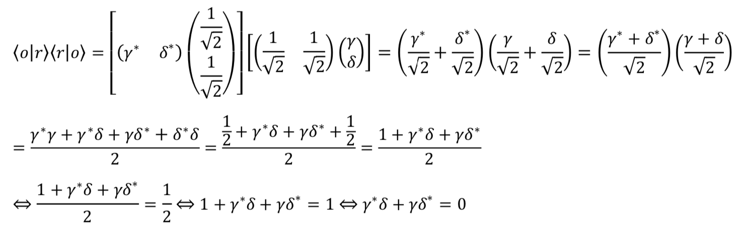
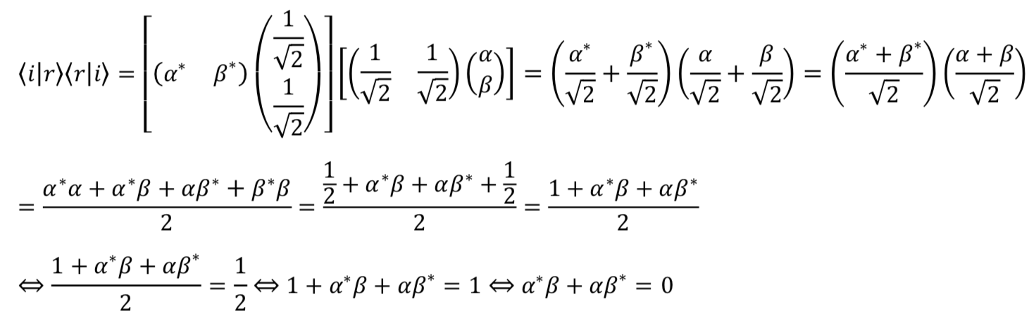
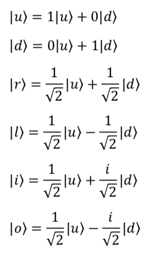
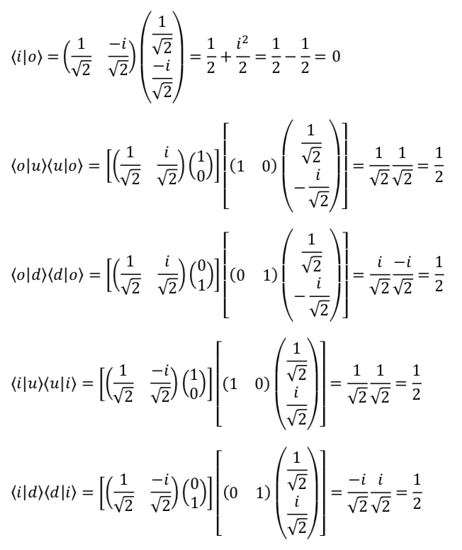
As with a spin prepared in the $+x$ or $-x$ directions, if we prepare a spin in either the $+y$ or $-y$ direction and measure in the $+z$ direction, then 50% of the time we will measure spin up (+1) and 50% of the time we will measure spin down (-1). Equations that describe such results are:

$\ket{i}=\frac{1}{\sqrt 2}\ket{u}+\frac{i}{\sqrt 2}\ket{d}$

and

$\ket{i}=\frac{1}{\sqrt 2}\ket{u}+\frac{i}{\sqrt 2}\ket{d}$

where $i=\sqrt{1}$ .

Notice that a portion of these expressions are complex. We’ve said that complex numbers are necessary to make the mathematical machinery of quantum mechanics work. The proof of this fact and the derivation of these equations is tedious. However, this proof and this derivation can be found by clicking .

These proofs are taken from Filip Van Lijsebetten. The original website from which they were taken is now defunct but they can still be found here (exercises 2.2 and 2.3):

We need to start by proving that use of complex numbers is necessary. To begin, let’s assume that we don’t know what the coefficients of $\ket{u}$ and $\ket{d}$ are. Then our expressions start out as

$\ket{i}=\alpha\ket{u} + \beta\ket{d}$

$\ket{o}=\gamma\ket{u} + \delta\ket{d}$

We know from experiments that if a spin is prepared in one spatial direction and measured in a spatial direction that is at $90^\circ$ to the direction of preparation (e.g., prepare in $x$ , measure in $z$ , then the probability of measuring +1 or -1 is $\frac12$ . This can be expressed mathematically as

The same is true if a spin is prepared in the $+y$ or $-y$ direction and measured in the $+x$ or $-x$ directions. Expressed mathematically,

$\braket{o}{r}\braket{r}{o}=\braket{o}{l}\braket{d}{l}=\braket{i}{r}\braket{r}{i}=\braket{i}{l}\braket{l}{i}=\frac12$

We can use the results from the calculations we performed above and obtain the following:

and

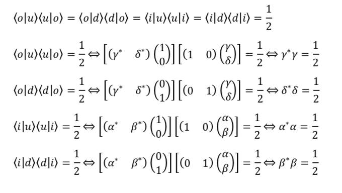
So $\alpha^*\beta + \alpha\beta^* = 0 \quad \Rightarrow \quad \alpha^*\beta=-\alpha\beta^*=-[(\alpha^*\beta)^*]$

Let $\alpha^*\beta=a+bi$ with $a,b\in\mathbb{R}$ . Then $(\alpha^*\beta)^*=a-bi$ .

It follows that

$a+bi--(a-bi)\,\Rightarrow\,a+bi=-a+bi\,\Rightarrow\,a=-a$

But the only way that this is possible is if $a=0$ . So $\alpha^*\beta=0+bi=bi$ . That means that $\alpha^*\beta$ is purely imaginary.

We could use similar arguments to show that $\gamma^*\delta$ is also purely imaginary.

But if $\alpha^*\beta$ is imaginary then $\alpha$ and $\beta$ cannot both be real. And if $\gamma^*\delta$ is purely imaginary, then $\gamma$ and $\delta$ cannot both be real. Why? Because 2 real numbers yields a real number, not an imaginary number. In fact, the only situations that work are if at least one of $\alpha-\beta$ or $\gamma-\delta$ is imaginary. Let’s examine the case of $\alpha^*\beta$ to illustrate this.

Let $\alpha$ and $\beta$ both be mixed real and imaginary numbers. For example, let $\alpha = a + bi$ and $\beta = c + di$ . Then $\alpha^*\beta=(a-bi)(c-di)=ac-adi-bci+bd$ which is mixed imaginary.

Next, let $\alpha$ and $\beta$ both be purely imaginary. For example, let $\alpha = bi$ and $\beta = di$ . Then $\alpha^*\beta=(-bi)(di)=bd$ which is real.

Finally, let one of $\alpha$ and $\beta$ be real and the other be mixed imaginary. For example, let $\alpha=a+bi$ and $\beta=di$ . Then $\alpha^*\beta=(a-bi)(di)=adi-bdi^2=adi-bd(-1)=adi+bd$ which is mixed imaginary.

So we’ve shown that some part of the expression for the state vector of a spin in the $y$ direction has to be imaginary. Now what we need to show is that the equations

$\ket{i}=\frac{1}{\sqrt 2}\ket{u}+\frac{i}{\sqrt 2}\ket{d}$

and

$\ket{o}=\frac{1}{\sqrt 2}\ket{u}-\frac{i}{\sqrt 2}\ket{d}$ (which incorporate imaginary numbers) fit the experimental data.

Hang on to your hats; here it goes.

Expressions for various state vectors in the z-basis are:

Expressions for state vectors in z-basis

Probabilities for a spin prepared either in the +y or -y directions to be measured as +1 in various directions are as follows:

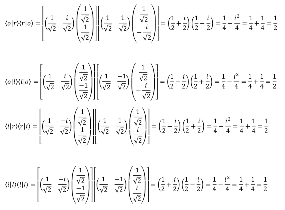
If we examine all of these equations carefully, we can see that they describe known experimental data perfectly.

Using these expressions for $\ket{i}$ and $\ket{o}$ , we can now construct the linear operator for spin y, $\sigma_y$ . The procedure is analogous to that used for finding the operators $\sigma_z$ and $\sigma_x$ .

$\begin{array}{rcl} \ket{i}&=&\frac{1}{\sqrt 2}\ket{u}+\frac{i}{\sqrt 2}\ket{d}\\ &=&\frac{1}{\sqrt 2}\mqty[1\\0]+\frac{i}{\sqrt 2}\mqty[0\\1]\\ &=&\mqty[\frac{1}{\sqrt 2}\\0] + \mqty[0 \\ \frac{i}{\sqrt 2}]\\ &=&\mqty[\frac{1}{\sqrt 2}\\\frac{i}{\sqrt 2}] \end{array}$

and

$\begin{array}{rcl} \ket{0}&=&\frac{1}{\sqrt 2}\ket{u}-\frac{i}{\sqrt 2}\ket{d}\\ &=&\frac{1}{\sqrt 2}\mqty[1\\0]-\frac{i}{\sqrt 2}\mqty[0\\1]\\ &=&\mqty[\frac{1}{\sqrt 2}\\0] - \mqty[0 \\ \frac{i}{\sqrt 2}]\\ &=&\mqty[\frac{1}{\sqrt 2} \\ -\frac{i}{\sqrt 2}] \end{array}$

Next, we use this information to write 2 eigenvalue equations:

$\mqty [(\sigma_y)_{11} & {(\sigma_y)}_{12} \\ {(\sigma_y)}_{21} & {(\sigma_y)}_{22}] \mqty[\frac{1}{\sqrt 2} \\ \frac{i}{\sqrt 2}] = +1\mqty[\frac{1}{\sqrt 2} \\ \frac{i}{\sqrt 2}]$

and

$\mqty[{(\sigma_y)}_{11} & {(\sigma_y)}_{12} \\ {(\sigma_y)}_{21} & {(\sigma_y)}_{22}] \mqty[\,\,\,\,\, \frac{1}{\sqrt 2} \\ -\frac{i}{\sqrt 2}] = -1\mqty[\,\,\,\,\, \frac{1}{\sqrt 2} \\ -\frac{i}{\sqrt 2}]$

We can translate these eigenvalue equations into 4 equations in 4 unknowns:

$\begin{array}{rcl} \frac{1}{\sqrt 2}(\sigma_y)_{11} + \frac{i}{\sqrt 2}{(\sigma_y)}_{12} &=& \,\,\,\,\, \frac{1}{\sqrt 2}\\ \, &\,& \, \\ \frac{1}{\sqrt 2}{(\sigma_y)}_{21} + \frac{i}{\sqrt 2}{(\sigma_y)}_{22} &=& \,\,\,\,\, \frac{i}{\sqrt 2}\\ \, &\,& \, \\ \frac{1}{\sqrt 2}{(\sigma_y)}_{11} - \frac{i}{\sqrt 2}{(\sigma_y)}_{12} &=& -\frac{1}{\sqrt 2}\\ \, &\,& \, \\ \frac{1}{\sqrt 2}{(\sigma_y)}_{21} - \frac{i}{\sqrt 2}{(\sigma_y)}_{22} &=& \,\,\,\,\, \frac{i}{\sqrt 2} \end{array}$

Adding the first and third equations gives us:

$\begin{array}{cccccc} & \frac{1}{\sqrt 2}(\sigma_y)_{11} & + & \frac{i}{\sqrt 2}{(\sigma_y)}_{12} &=& \frac{1}{\sqrt 2}\\ + & \frac{1}{\sqrt 2}{(\sigma_y)}_{11} & - & \frac{i}{\sqrt 2}{(\sigma_y)}_{12} & = & -\frac{1}{\sqrt 2}\\ \hline &(\frac{1}{\sqrt 2} + \frac{1}{\sqrt 2}){(\sigma_y)}_{11} &+& (\frac{i}{\sqrt 2} - \frac{i}{\sqrt 2}){(\sigma_y)}_{12} &=& \frac{1}{\sqrt 2} - \frac{1}{\sqrt 2}\\ \, & \, & \, & \, & \, & \, \\ & (\frac{1}{\sqrt 2} + \frac{1}{\sqrt 2}){(\sigma_y)}_{11} &+& 0 &= &0 \\ & {(\sigma_y)}_{11} &\,& \, &= &0 \end{array}$

Substituting ${(\sigma_x)}_{11}=0$ back into the first equation gives:

$0 &+& (\frac{i}{\sqrt 2}){(\sigma_y)}_{12} &=& \frac{1}{\sqrt 2}$

Multiply both sides by $i\sqrt{2}$ . We get:

$\begin{array}{rcl} i\,\cancel{\sqrt{2}}(\frac{i}{\cancel\sqrt 2}){(\sigma_y)}_{12}&=& i\,\cancel{\sqrt{2}}\frac{1}{\cancel{\sqrt 2}}\\ -{(\sigma_y)}_{12}&=&i\\ {(\sigma_y)}_{12}&=&-i \end{array}$

Next, add the second and fourth equations. That yields

$\begin{array}{cccccc} & \frac{1}{\sqrt 2}(\sigma_y)_{21} & + & \frac{i}{\sqrt 2}{(\sigma_y)}_{22} &=& \frac{1}{\sqrt 2}\\ + & \frac{1}{\sqrt 2}{(\sigma_x)}_{21} & - & \frac{i}{\sqrt 2}{(\sigma_y)}_{22} & = & \frac{i}{\sqrt 2}\\ \hline &(\frac{1}{\sqrt 2} + \frac{1}{\sqrt 2}){(\sigma_y)}_{11} &+& (\frac{i}{\sqrt 2} - \frac{i}{\sqrt 2}){(\sigma_y)}_{12} &=& \frac{i}{\sqrt 2} + \frac{i}{\sqrt 2}\\ \, & \, & \, & \, & \, & \, \\ & (\frac{1}{\sqrt 2} + \frac{1}{\sqrt 2}){(\sigma_y)}_{21} &+& 0 &= &\frac{i}{\sqrt 2} + \frac{i}{\sqrt 2} \\ \end{array}$

We are left with

$\frac{2}{\sqrt{2}}\sigma_y=\frac{2}{\sqrt{2}}i$

Multiply both sides of this equation by $\frac{\sqrt{2}}{2}$ . That leaves

${(\sigma_y)}_{21} = i$

Substituting ${(\sigma_y)}_{21}=i$ back into the second equation gives:

$\frac{1}{\sqrt{2}}i + \frac{i}{\sqrt{2}}\sigma_{y_{22}} = \frac{i}{\sqrt{2}}$

Divide through by $\frac{i}{\sqrt{2}}$ . That gives us

$i + {(\sigma_y)}_{22} = i$

Subtract $i$ from both sides. We get

${(\sigma_y)}_{22} = 0$

So our $\sigma_y$ matrix is:

$\sigma_y=\mqty[0&-i\\i&0]$

Summary: Pauli matrices

To summarize, there are three matrices, called the Pauli matrices, that represent the 3 operators associated spin in the 3 spatial directions: $\sigma_z$ , $\sigma_x$ , $\sigma_y$ . As we have seen, they are:

$\sigma_z=\mqty[1&0\\0&-1] \quad \sigma_x=\mqty[0&1\\1&0] \quad \sigma_y=\mqty[0&-i\\i&0]$

As Susskind notes in his book

Operators are things that we use to calculate eigenvalues and eigenvectors.
Operators act on state vectors (which are abstract mathematical objects), not on actual physical systems.
When an operator acts on a state vector, it produces a new state vector.

However, it is important to realize that operating on a state vector is not the same as making a measurement.

The result of an operator operating on a state vector is a new state vector.
A measurement, on the other hand, is the result obtained when an apparatus interacts with a physical system. In the case of spin, for example, it is +1 or -1 .
The result of an operator operating on a state vector (i.e. a new state vector) is definitely not the same as the result of a measurement (for example, the +1 or -1 obtained when a spin is measured).
The state that results after an operator operates on a state vector is different than the state resulting after a measurement.

Here is an example of the latter. Suppose we prepare a spin in the $+x$ direction and measure it with our apparatus pointed in the $+z$ direction.

The state, $\ket{r}$ , that describes an electron spin prepared in the $+x$ direction and measured in the $+z$ direction is

$\ket{r}=\frac{1}{\sqrt 2}\ket{u} + \frac{1}{\sqrt 2}\ket{d}$

Acting on this state vector with $\sigma_z$ gives us

$\begin{array}{rcl} \sigma_z \ket{r} &=& \frac{1}{\sqrt 2}\sigma_z\ket{u} + \frac{1}{\sqrt 2}\sigma_z\ket{d}\\ &=& \frac{1}{\sqrt 2} \mqty[1&0\\0&-1] \mqty[1\\0] + \frac{1}{\sqrt 2} \mqty[1&0\\0&-1] \mqty[0\\1]\\ &=& \frac{1}{\sqrt 2} \mqty[1\\0] + \frac{1}{\sqrt 2} \mqty[0\\-1]\\ &=& \frac{1}{\sqrt 2} \mqty[1\\0] - \frac{1}{\sqrt 2} \mqty[0\\1]\\ &=& \frac{1}{\sqrt 2}\ket{u} - \frac{1}{\sqrt 2}\ket{d} \end{array}$

But this is definitely not the state that results from a measurement. The state that the spin is left in after a measurement would be $\ket{u}$ if the measurement is +1 or $\ket{d}$ if the measurement is -1.

So what does this new state vector that results after an operator operates on an original state vector have to do with measurement? It allows us to calculate the probability of each possible outcome of a measurement.

Deriving σ _n

The original experimental results we sought to describe mathematically were

the probabilities of a spin being measured as spin up (+1) and spin down (-1) given 1) that the spin was prepared in the x-z plane at $30^\circ$ clockwise from the z-axis and 2) that our measuring apparatus is oriented in the $+z$ direction .

To figure this out, what we’ll do is construct an operator that is associated with measurement of a spin oriented at any direction in space. We can represent the direction in space in which to measure as $\hat{n}$ which is a unit vector and has components $n_x$ , $n_y$ and $n_z$ . We won’t go through a formal proof of it but the operator associated with measurement of spin in the direction $\hat{n}$ (which we’ll call $\sigma_n$ ) behaves like a vector. Therefore, we can say

$\sigma_n = \sigma \cdot \hat{n} = \sigma_x n_x + \sigma_y n_y + \sigma_z n_z$

where the $n's$ are just numbers. Therefore:

$\begin{array}{rcl} \sigma_n &=& \mqty[0&1\\1&0] n_x + \mqty[0&-i\\i&0] n_y+ \mqty[1&0\\0&-1] n_z \\ &=& \mqty[0&n_x\\n_x&0] + \mqty[0&-in_y\\in_y&0] + \mqty[n_z&0\\0&-n_z] \\ &=& \mqty[n_z&n_x-in_y\\n_x+in_y&-n_z] \end{array}$

To solve our problem, we’ll need to find the eigenvalues and eigenvectors of our matrix, $\sigma_n$ . Also, we’ll use spherical coordinates. A quick visual review of spherical coordinates and reminder of how they relate to Cartesian coordinates is given in the following diagram:

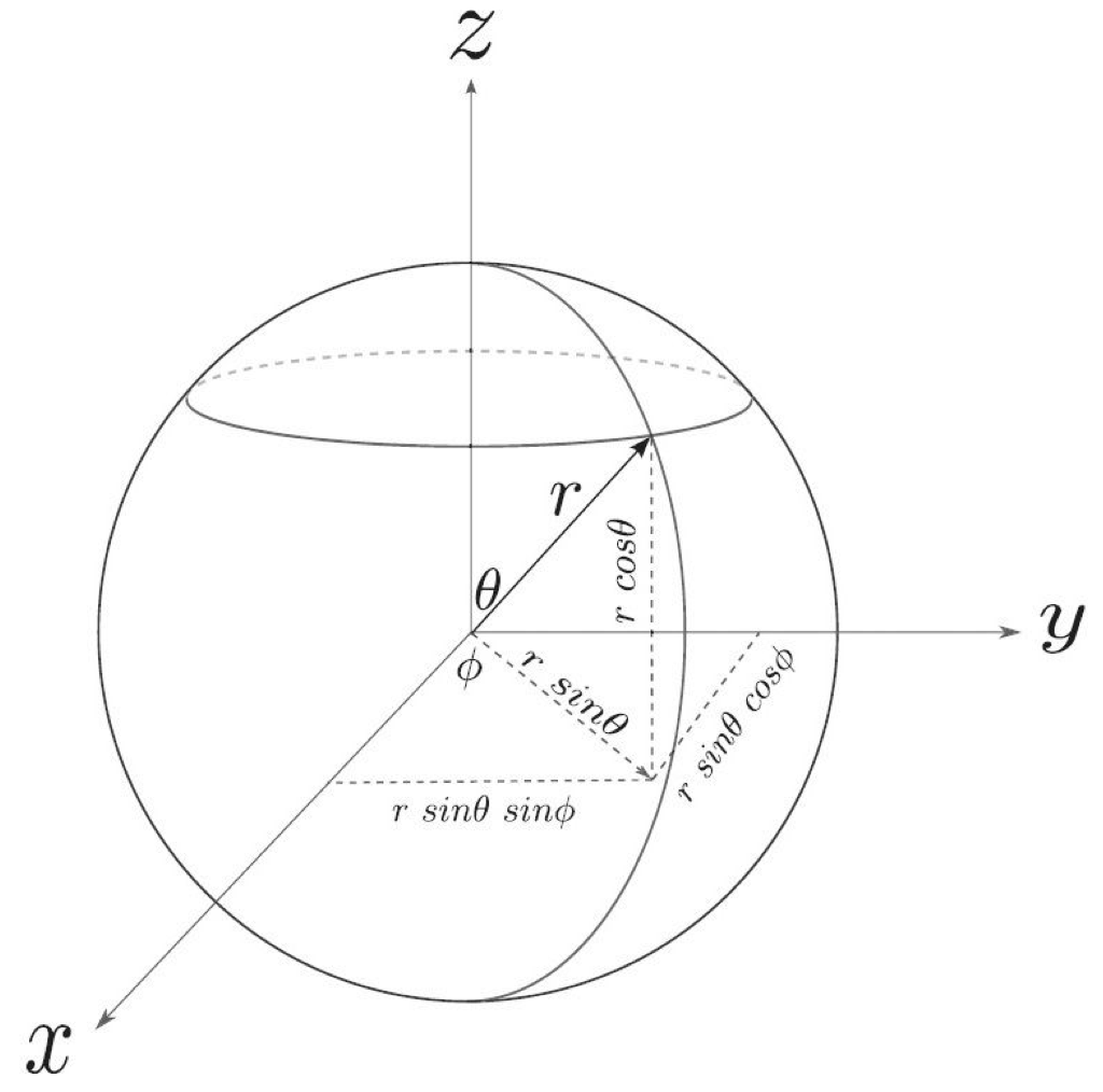
We’re dealing with a unit vector, $\hat{n}$ . Therefore $r=1$ . So, from the diagram,

$\n_x=\sin\theta \cos\phi$
$n_y=\sin\theta \sin\phi$
$n_z=\cos\theta$

Substituting the above values into $\sigma_n$ , we get:

$\sigma_n=\mqty[\cos\theta & \sin\theta \cos\phi-i\sin\theta \sin\phi\\\sin\theta \cos\phi+i\sin\theta \sin\phi & -\cos\theta]$

Since we’re dealing with an $\hat{n}$ that is in the x-z plane,

$\cos\phi = \cos 0 = 1$
$\sin\phi = \sin 0 = 0$

Substituting these values into $\sigma_n$ , we have:

$\begin{array}{rcl} \sigma_n=\sigma_n&=&\mqty[\cos\theta & \sin\theta \cos\phi-i\sin\theta \sin\phi\\\sin\theta \cos\phi+i\sin\theta \sin\phi & -\cos\theta]\\ \, &\,& \, \\ &=& \mqty[\cos\theta & (\sin\theta)(1)-(i\sin\theta) (0)\\ (\sin\theta) (1)+(i\sin\theta)(0) & -\cos\theta]\\ \, &\,& \, \\ &=&\mqty[\cos\theta & \sin\theta \\ \sin\theta & -\cos\theta] \end{array}$

If $\phi \neq 0$ , then the calculations become more complicated. To see these calculations, click

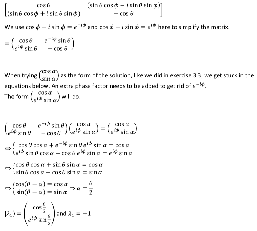
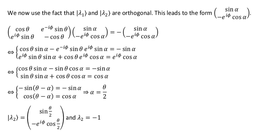
Continuing with our current simpler problem, calculation of the eigenvalues and eigenvectors of $\sigma_n$ goes as follows:

Our matrix $\sigma_n$ is filled with sines and cosines. Therefore, our eigenvectors $\ket{\lambda_1}$ and $\ket{\lambda_2}$ (which we’ll, at first, collectively refer to as $\ket{\lambda}$ ) are likely to be something like $\mqty[\cos\alpha \\ \sin\alpha]$ . We don’t know $\alpha$ ; the is what we have to find – in terms of $\theta$ . So we write eigenvalue equations:

$\begin{array}{rcl} \sigma_n \ket{\lambda}&=& \lambda\ket{\lambda}\\ \, &\,& \, \\ \mqty[\cos\theta & \sin\theta\\ \sin\theta & -\cos\theta]\mqty[\cos\alpha \\ \sin\alpha]&=&\lambda\mqty[\cos\alpha \\ \sin\alpha] \end{array}$

Doing matrix multiplication leaves us with 2 equations in 2 unknowns:

$\cos\theta \cos\alpha + \sin\theta \sin\alpha = \lambda \cos\alpha$

and

$\sin\theta \cos\alpha - \cos\theta \sin\alpha = \lambda \sin\alpha$

From the page on this site entitled Trigonometry Identities, we know that

$\cos\theta \cos\alpha + \sin\theta \sin\alpha = \cos (\theta - \alpha)$
$\sin\theta \cos\alpha - \cos\theta \sin\alpha = \sin (\theta - \alpha)$

$\cos (\theta - \alpha) = \lambda \cos\alpha$
$\sin (\theta - \alpha) = \lambda \sin\alpha$

Divide both sides of the top equation by $\cos\alpha$ and both sides of the bottom equation by $\sin\alpha$ . That gives us

$\frac{\cos (\theta - \alpha)}{\cos\alpha} = \lambda$
$\frac{\sin (\theta - \alpha)}{\sin\alpha} = \lambda$

The left-hand side of both of the above equations equal $\lambda$ . Therefore, they are equal to each other:

$\frac{\cos (\theta - \alpha)}{\cos\alpha} = \frac{\sin (\theta - \alpha)}{\sin\alpha}$

Multiply both sides of this equation by $\cos\alpha \sin\alpha$ . We get

$\cos (\theta - \alpha) \sin\alpha = \sin (\theta - \alpha) \cos\alpha$

Subtract $\sin (\theta - \alpha) \cos\alpha$ from both sides. That leaves us with

$\cos (\theta - \alpha) \sin\alpha - \sin (\theta - \alpha) \cos\alpha = 0$

Let $\beta = \theta - \alpha$ . Substituting this into the above equation gives us

$\cos \beta \sin\alpha - \sin \beta \cos\alpha = 0$

Using our trigonometry identities again

$\cos \beta \sin\alpha - \sin \beta \cos\alpha = sin(\alpha - \beta)$

But $\beta = \theta - \alpha$ . Thus,

$\sin[\alpha - (\theta - \alpha)] = \sin(2\alpha-\theta)=0$

We know that there are 2 conditions in which $\sin(x) = 0$ :

$x = 0$
$x = \pi$

It follows, then, that $\sin(2\alpha-\theta)=0$ when

$2\alpha-\theta = 0 \quad \Rightarrow \quad \alpha = \frac{\theta}{2}$
$2\alpha-\theta = \pi \quad \Rightarrow \quad \alpha = \frac{\theta}{2} + \frac{\pi}{2}$

So that leaves us with the opportunity to calculate 2 eigenvalues, which is what we want. Recall that

$\frac{\cos (\theta - \alpha)}{\cos\alpha} = \lambda$
$\frac{\sin (\theta - \alpha)}{\sin\alpha} = \lambda$

We’ll arbitrarily use the top equation to calculate our eigenvalues and eigenvectors.

First,

$\lambda_1 = \frac{\cos (\theta - \alpha)}{\cos\alpha} = \frac{\cos(\theta - \frac{\theta}{2})}{\cos \frac{\theta}{2}}=\frac{\cos \frac{\theta}{2}}{\cos \frac{\theta}{2}}=+1$

and

$\ket{\lambda_1} = \mqty[\cos\alpha \\ \sin\alpha] = \mqty[\cos\frac{\theta}{2} \\ \sin\frac{\theta}{2}]$

Second,

$\lambda_1 = \frac{\cos (\theta - \alpha)}{\cos\alpha} = \frac{\cos (\theta - \frac{\theta}{2} - \frac{\pi}{2})}{\cos (\frac{\theta}{2} + \frac{\pi}{2})}=\frac{\cos (\frac{\theta}{2} - \frac{\pi}{2})}{\cos (\frac{\theta}{2} + \frac{\pi}{2})}$

To solve the last step in the above equation, we need to figure out alternative expressions for $(\frac{\theta}{2} - \frac{\pi}{2})$ and $(\frac{\theta}{2} + \frac{\pi}{2})$ . To do this, we need to use the following trigonometry identities:

$\cos(\frac{\pi}{2} - \theta) = sin \theta$
$\cos(\frac{\pi}{2} + x) = -sin \theta$

Thus,

$\lambda_1 = \frac{\cos (\frac{\theta}{2} - \frac{\pi}{2})}{\cos (\frac{\theta}{2} + \frac{\pi}{2})} = \frac {\sin \theta}{-\sin \theta} = -1$

Now for the eigenvector:

$\ket{\lambda_2} = \mqty[ \cos (\frac{\theta}{2} + \frac{\pi}{2}) \\ \sin (\frac{\theta}{2} + \frac{\pi}{2}) ]$

To solve this equation, we have to find expressions for $\cos (\frac{\theta}{2} + \frac{\pi}{2})$ and $\sin (\frac{\theta}{2} + \frac{\pi}{2})$ . To do this, we let $x = \frac{\theta}{2}$ and use the Trigonometry Identities

$\cos (x + \frac{\pi}{2}) = -\sin x$
$\sin (x + \frac{\pi}{2}) = \cos x$

When we do this, we get

$\ket{\lambda_2} = \mqty[ \cos (\frac{\theta}{2} + \frac{\pi}{2}) \\ \sin (\frac{\theta}{2} + \frac{\pi}{2}) ] = \mqty [ -\sin \frac{\theta}{2} \\ \cos \frac{\theta}{2}]$

Now that we’ve got the eigenvalues and eigenvectors, we can calculate the probability of measuring spin up, $P(+1)$ , as follows:

$\begin{array}{rcl} P(+1)&=&\braket{\lambda_1}{u}\braket{u}{\lambda_1}\\ &=& \mqty[\cos\frac{\theta}{2} & \sin\frac{\theta}{2}]\mqty[1\\0]\mqty[1&0]\mqty[1&0]\mqty[\cos\frac{\theta}{2} \\ \sin\frac{\theta}{2}] \\ &=& \cos\frac{\theta}{2} \cdot \cos\frac{\theta}{2} \\ &=& (\cos\frac{\theta}{2})^2 \end{array}$

We calculate the probability of measuring spin down, $P(-1)$ , in a similar fashion:

$\begin{array}{rcl} P(-1)&=&\braket{\lambda_2}{u}\braket{u}{\lambda_2}\\ &=& \mqty[-\sin\frac{\theta}{2} & \cos\frac{\theta}{2}]\mqty[1\\0]\mqty[1&0]\mqty[-\sin\frac{\theta}{2} & \cos\frac{\theta}{2}] \\ &=& -\sin\frac{\theta}{2} \cdot -\sin\frac{\theta}{2} \\ &=& (\sin\frac{\theta}{2})^2 \end{array}$

Finally, we prepare our spin in the direction $30^\circ$ from the =z-axis toward the +x-axis. Then we measure in the +z direction which is $\theta=-30^\circ$ . We already have expressions for $P(+1)$ and $P(-1)$ . Now all we have to do is plug $\theta=-30^\circ$ into those expressions. When we do, we obtain:

$P(+1)=\cos^2\frac{\theta}{2}=\cos^2\frac{30}{2}=\cos^{2} 15=0.966^2=0.933$

and

$P(-1)=\sin^2\frac{\theta}{2}=\sin^2\frac{30}{2}=\sin^{2} 15=0.259^2=0.067$

We haven’t discussed it previously but if we repeat this experiment an infinite number of times, then the average value of our measurements (called the expectation value) will be what would be predicted by classical mechanics. Experimental data indicates that, for spin, that this expectation value is given by the cosine of the angle between the direction at which the spin is prepared and the direction at which it is measured. The mathematical expression for the expectation value is to enclose the entity to be measured (which is an operator, also called an observable) in brackets. In our case, the angle of between preparation and measurement is $-30^\circ$ . Therefore, experiments suggest that the exception value should be $\cos (-30) = 0.866$ . Let’s now see if our mathematical predictions match the experimental results.

The formula for the expectation value of an observable, $L$ , in quantum mechanics is just the same as the general formula for average value; we multiply the value of each measurement times the probability of its occurrence then take the sum of each of these products:

$\left<L\right>=\displaystyle\sum_i \lambda_i P(\lambda_i)$ where

$\lambda_i$ are the eigenvalues (i.e., the value of the measurements)
$P(\lambda_i)$ are the probabilities of occurrence of each $\lambda_i$

So,

$\begin{array}{rcl} \left<\sigma_n\right>&=&(+1)(\cos\frac{\theta}{2})^2 + (-1)(\sin\frac{\theta}{2})^2 \\ &=& (\cos\frac{\theta}{2})^2 - (\sin\frac{\theta}{2})^2 \end{array}$

There is another trigonometry identity that states

$(\cos\frac{\theta}{2})^2 - (\sin\frac{\theta}{2})^2 = \cos \theta$

Therefore,

$\left<\sigma_n\right> = \cos \theta = \cos 30 = 0.866$

just as we had hoped.

We could also plug in the values we got for $(\cos\frac{\theta}{2})^2$ and $(\sin\frac{\theta}{2})^2$ . When we do, we get

$\begin{array}{rcl} \left<\sigma_n\right> &=& (\cos\frac{\theta}{2})^2 - (\sin\frac{\theta}{2})^2 \\ &=& 0.933 - 0.067 = 0.866 \end{array}$

again, agreeing with experiment.

Other operators and wave functions

We’ve spoken so far about a simple physical system – spin. However, the mathematical tools that describe spin are the same ones that are used in other physical systems. Therefore, we examined this system in detail so that readers who are completely new to this subject have some idea about what we are talking about when we discuss these things – especially operators and wave functions – in what follows.

When we talked about spin, we talked about a discrete system. That is, the vectors used to describe states and wave functions, for example, had a finite number of dimensions, namely 2. Likewise, operators (or observables) were matrices with a finite number of entries. However, continuous functions can form vector spaces like discrete vectors. The difference is that functions have an infinite number of dimensions.

The observables we’ll be talking about in our proofs of the equations of Bohmian mechanics, and the operators that represent them, are involved with continuous variables. Specifically, they are position, momentum and energy. We’ll examine each one, in turn.

Position

By position, we mean position in space. Of course, position is a continuous variable. We’ll call the operator that’s involved in the measurement of position $\mathbf{X}$ . When it acts on a wave function, what it does is multiply the wave function by the value of a position in space, which we’ll call $x$ . So

$\mathbf{X}\psi(x) = x\psi(x)$

We need to examine the eigenvalues and eigenstates of the position operator. The eigenvalue equation is

$\mathbf{X}\ket{\psi} = x_0\ket{\psi}$

In terms of wave functions, this becomes:

$x\psi(x) = x_0\psi(x)$

Rearranging, we get

$(x-x_0)\psi(x) = 0$

For this equation to be true, either $(x-x_0)$ or $\psi(x)$ must be zero. The case where $\psi(x)$ is the zero vector is uninteresting. We want to evaluate the case where $\psi(x)\neq 0$ . This only happens when

$(x-x_0) = 0 \quad \Rightarrow \quad x=x_0$

So for $\psi(x)$ to be nonzero, $x$ is zero at every position except one: $x_0$ . This sounds a lot like the Dirac delta function, $\delta$ .

The Dirac delta function is a function that has no width along the x-axis, is infinitely high in the y-direction and has an area of 1 under it (i.e., it is infinitely concentrated at one point along the x-axis). $\delta(0)$ is infinitely concentrated at $x=0$ . Therefore, $\delta(x-x_0)$ is infinitely concentrated at $x=x_0$ . (This is because $x-x_0 = 0$ which makes $\delta(x-x_0)=\delta(0)$ ).

The eigenstate (or in this instance, eigenfunction) of $\mathbf{X}$ , then, is

$\psi(x)=\delta(x-x_0)$

This makes sense since, by definition, an eigenstate or eigenfunction is the state/function where the outcome of a measurement is – with 100% certainty – its associated eigenvalue.

We can make the same argument for eigenvalues $x_1, x_2, x_3\dots$ , indeed, for every point on the x-axis. So every point on the x-axis is an eigenvalue.

Wave functions that are not eigenfunctions must specify a probability amplitude for every eigenvalue. Since every point on the x-axis is an eigenvalue, such a wave function must specify a probability amplitude for a particle to be found at every point on the x-axis. There are an infinite number of x-axis points, thus, the wave functions for position are continuous functions.

Momentum

Momentum, in quantum mechanics, is a little more complicated than position. Specifically, the connection between the momentum operator in quantum mechanics and the classical notion of momentum (i.e., $p=mv$ ) is less intuitive than the relationship between the quantum position operator and its classical counterpart. However, with some work, the connection will become apparent.

The quantum momentum operator is

$\mathbf{P} = -i\bar{h}\mathbf{D} = -i\bar{h}\frac{d}{dx}$

To prove that it is a quantum operator, we have to prove 2 things:

$\mathbf{P}$ is a linear operator
$\mathbf{P}$ is a Hermitian operator

We’ll prove each in turn. The way that we’ll do this is to prove the above properties for the differential operator, $\mathbf{D}$ . Because $\mathbf{P}$ is just $\mathbf{D}$ multiplied by a constant, the properties that apply to $\mathbf{D}$ also apply to $\mathbf{P}$ .

Proof: P is linear

This proof is copied directly from the following link (exercise 8.1):

https://onedrive.live.com/?authkey=%21AAM3H%2DTDeYaAbaI&cid=21D08FA0C16B93A5&id=21D08FA0C16B93A5%2128241&parId=21D08FA0C16B93A5%215777&o=OneUp

Proof: p is hermitian

This proof is taken from Susskind and Friedman, Quantum Mechanics: The Theoretical Minimum, chapter 8.

We note that, if an operator $\mathbf{L}$ is Hermitian, and we sandwich it between a bra and a ket vector, then the quantities we get should be complex conjugates of each other:

$\bra{\Psi}\mathbf{L}\ket{\Phi} = \bra{\Phi}\mathbf{L}\ket{\Psi}^*$

Notice that uppercase $\Psi$ and $\Phi$ are used in this equation while lowercase $\psi$ and $\phi$ are used elsewhere. Susskind and Friedman use capital Greek letters to represent state vectors and lower case Greek letters to represent wave functions, which they define as being a state vector expressed in a given basis (which is determined by and operator. I’m not certain that it makes a difference in this proof but they use this convention in there proof so we’ll just roll with it here.

Anyway let’s start by check to see of this works with the position operator, $\mathbf{X}$ .

Recalling that

$\mathbf{X}\psi(x) = x\psi(x)$

we find the following to be true:

$\bra{\Psi}\mathbf{X}\ket{\Phi} = \int \psi^*(x)\, x\, \phi(x)\,dx$

and

$\bra{\Phi}\mathbf{X}\ket{\Psi} = \int \phi^*(x)\, x\, \psi(x)\,dx$

Because $x$ is real, the above integrals are complex conjugates of each other, and therefore, $\mathbf{X}$ is Hermitian.

What about $\mathbf{D}$ ? We have

$\bra{\Psi}\mathbf{D}\ket{\Phi} = \int \psi^*(x)\,\frac{d\phi(x)}{dx}\,dx$

and

$\bra{\Phi}\mathbf{D}\ket{\Psi} = \int \phi^*(x)\,\frac{d\psi(x)}{dx}\,dx$

In this form, we cannot definitively determine whether the above integrals are complex conjugates of each other. We need to make a direct comparison. To do this, we need to make use of integration by parts. Here is a quick review of this technique:

$\begin{array}{rcl} d(FG) &=& F\,dG + G\,dF\\ \int d(FG) &=& \int F\,dG + \int G\,dF\\ \eval{FG}_a^b &=& \int F\,dG + \int G\,dF\\ \end{array}$

State and wave functions are normalized. Thus, they must go to zero at infinity. Integrals of such wave function span entire axises meaning the limits of integration are from $-\infty$ to $+\infty$ . Therefore, $\displaystyle\int _{-\infty}^{+\infty} d(FG) = \eval{FG}_0^0 = 0$ . So the term $\int d(FG)$ “disappears” and we’re left with

$0 = \int F\,dG + \int G\,dF \,\, \Rightarrow \,\, -\int F\,dG = \int G\,dF$ or $\int F\,dG = -\int G\,dF$ .

Applying this to our original problem, let

$F$ be analogous to $\phi^*$
$G$ be analogous to $\psi$

Then,

$\begin{array}{rcl} d(\phi^*\psi) &=& \phi^*\,d\psi + \psi\,d\phi^*\\ \displaystyle\int _{-\infty}^{+\infty} d(\phi^*\psi) &=& \displaystyle\int _{-\infty}^{+\infty} \phi^*\,d\psi + \displaystyle\int _{-\infty}^{+\infty}\psi\,d\phi^*\\ \eval{\phi^*\psi}_{-\infty}^{+\infty} = &=& \displaystyle\int _{-\infty}^{+\infty} \phi^*\,d\psi + \displaystyle\int _{-\infty}^{+\infty}\psi\,d\phi^*\\ 0 &=& \displaystyle\int _{-\infty}^{+\infty} \phi^*\,d\psi + \displaystyle\int _{-\infty}^{+\infty}\psi\,d\phi^*\\ -\displaystyle\int _{-\infty}^{+\infty}\psi\,d\phi^* &=& \displaystyle\int _{-\infty}^{+\infty} \phi^*\,d\psi \end{array}$

So now we have

$\bra{\Psi}\mathbf{D}\ket{\Phi} = \int \psi^*(x)\,\frac{d\phi(x)}{dx}\,dx$

and

$\bra{\Phi}\mathbf{D}\ket{\Psi} = -\int \psi\,\frac{d\phi^*}{dx}\,dx$

From this, we can see that

$\bra{\Psi}\mathbf{D}\ket{\Phi} = -\bra{\Phi}\mathbf{D}\ket{\Psi}^*$

In other words,

$\mathbf{D}^\dag = -\mathbf{D}$

instead of

$\mathbf{D}^\dag = \mathbf{D}$

which would be the case if $\mathbf{D}$ were Hermitian. To make it Hermitian, we would need to change $\mathbf{D}$ to $i\mathbf{D}$ .

Why? We know from the above argument that

$\mathbf{D^\dag}=-\mathbf{D}$

Now multiply $\mathbf{D}$ by $i$ and take the transpose:

$(i\mathbf{D})^\dag = i^*\mathbf{D^\dag} = -i(-\mathbf{D}) = i\mathbf{D}$

So we have $(i\mathbf{D})^\dag = i\mathbf{D}$ which, by definition, makes $\mathbf{D}$ Hermitian.

Quantum Momentum operator

However, if we assume that the quantum momentum operator approaches the classical notion of momentum, then the units of the quantum momentum operator should be the same as those of momentum in classical physics. If so, then $iD$ doesn’t fit the bill.

Let,

L = length
M = mass
T = time

The units of $iD$ are $i\frac{d}{dx}\,\,\Rightarrow\,\,\frac{1}{L}$ . The units of momentum are $p=mv\,\,\Rightarrow\,\,M\frac{L}{T}$ . To make them the same, we multiply $iD$ by Planck’s constant, $\hbar$ , which has units $\frac{ML^2}{T}$ . We have

$i\hbar\frac{d}{dx}\,\,\Rightarrow\,\,\frac{ML^2}{T}\cdot\frac{1}{L}=M\frac{L}{T}$

which, of course, are the units of momentum in classical physics. So the momentum operator in quantum mechanics is

$i\hbar \mathbf{D} = i\hbar \frac{d}{dx}$

Energy

The total energy of a system in classical mechanics is given by the Hamiltonian. Similarly, the linear operator for energy in quantum mechanics is the quantum Hamiltonian. Its form varies with the type of physical system we’re considering. For example,

The quantum Hamiltonian for a harmonic oscillator (i.e., a system that behaves like a mass attached to a spring) is:

$\mathbf{H} = \frac{\mathbf{P^2}}{2m}+\frac12 m\omega^2\mathbf{X}$ where

$\mathbf{H}$ is the quantum Hamiltonian
$\mathbf{P}$ is the quantum operator for momentum
$m$ is mass
$\omega=\sqrt{\frac{k}{m}}$
$k$ is the spring constant
$\mathbf{X}$ is the position operator

The quantum Hamiltonian for a charged particle in an electromagnetic field is:

$\mathbf{H} = \frac{1}{2m}(-i\hbar\nabla-q\mathbf{A})^2 + q\phi$

I won’t even tell you what all of these symbols mean because it’s not important for our discussion here – you get the picture.

However, what is important to our derivation of Bohmian mechanics is the quantum operator for a particle moving in a potential energy field. In this case the potential is generic – it could be any kind of potential energy. Like many quantum Hamiltonians, it is similar to the classical Hamiltonian for the specific quantity it represents. It is given by:

$\mathbf{H} = \frac{1}{2}mv^2 + V(\mathbf{x},t) = \frac{\mathbf{P^2}}{2m} + \mathbf{V}(\mathbf{x},t)$ where

$\mathbf{H}$ , $m$ and $\mathbf{P}$ are as defined above
$\mathbf{x}$ is a vector that represents position; it could be in the x, y or z direction
$t$ is time
$\mathbf{V}$ is the potential energy, which depends on both spatial position and time; it, itself, is an operator that multiplies whatever it acts upon by the potential energy at position $\mathbf{x}$ and time, $t$

It should be noted that, in the strict Schrodinger formulation of quantum mechanics, the Hamiltonian is constant and state vectors(functions) vary with time. By contrast, in the Heisenberg formulation, the Hamiltonian varies with time and state vectors(functions) are constant. However, there are hybrid versions in which the Hamiltonian and/or state function vary with time. These formulations are all equivalent. Bohm, in his derivation, uses a hybrid version in which position and potential energy both vary with position and time.

Contents